20 RL Debugging and Direct Policy Search
Lecture 20
reinforcement learning debugging, direct policy search, REINFORCE, policy gradient, POMDPs
Lecture video: Lecture 20: RL Debugging and Diagnostics · 1:12:43
Based on the lecture by Andrew Ng — CS229, Stanford University, Autumn 2018.
Every reinforcement-learning method in the course so far has been indirect: estimate the value function, then read the policy off it with an argmax. The last lecture introduces the other family. Direct policy search writes the policy down as a parametrised function, the way logistic regression writes down a hypothesis, and tunes its parameters by gradient ascent on the expected payoff, never computing a value function at all. The algorithm Ng derives, REINFORCE, gets an unbiased estimate of that gradient from a single run of the system. Unbiased is not the same as useful: the estimate is so noisy that REINFORCE is notoriously slow, and part of that noise comes from terms that average to zero and can be dropped. Before any of that, Ng finishes a promise from lecture 12 and restates the helicopter diagnostics in the notation the course has since introduced.
20.1 Debugging the helicopter, in RL notation
4:05 Lecture 12 walked through the diagnostics for Ng’s autonomous helicopter before the course had any reinforcement learning to describe them with (Section 12.5). The setup is now familiar. Build a simulator, a learned model or something richer, as in Section 18.3. Choose a reward function, such as the negative squared distance from where the helicopter should be. Run a reinforcement-learning algorithm on the finite-horizon problem to get a policy that maximises in the simulator. The first time, the controller flies much worse than the human pilot, and there are three things to try: improve the simulator, change the reward, or improve the RL algorithm. Ng is concrete about the last one. It means changing the discretization of a continuous state, or replacing the linear function approximator in fitted value iteration with a richer one such as a neural network.
The diagnostics are those of lecture 12 with the sign turned round, since the algorithm now maximises a payoff rather than minimising a cost. If flies well in simulation and badly in reality, the simulator is at fault. Otherwise, 8:28 record the human pilot’s flight and score it with the same reward. If the human’s payoff is higher, the algorithm failed to maximise the sum of rewards, because here is a policy that does better. If the algorithm’s payoff is higher and it still flies worse, maximising this reward is not the same as flying well, and the reward is what needs work.
13:12 A student asks whether the tests have an order. Ng checks the simulator first and turns to the other two only once it seems adequate. He also qualifies the whole procedure: the diagnostics look like a rigid decision rule, but in practice the answers are graded. The simulator is “kind of good”, the human beats the algorithm by a little, and the team looks at all three pieces of evidence together and decides where the next month goes. What he insists on is that the bottleneck moves as the project progresses, so the diagnostics are re-run after each round of work rather than once, and teams that prioritise this way move faster than teams that go by gut feel.
20.2 Searching for the policy directly
17:01 Ng shows one more example of the indirect route first. Zico Kolter’s quadruped crossing rough terrain relied on an approximate value function that scored, for a given height map of the terrain, how good each position of the robot was; the robot moved towards higher value. That is value iteration’s way of thinking: learn , or an approximation to it, then act greedily with (Section 17.4 and Section 18.5).
18:25 Direct policy search goes straight for the policy, with no value function in between. Its first step is the same as the first step of supervised learning. When logistic regression was introduced, Ng recalls, the form was pulled out of a hat (Section 3.5), and the learning algorithm’s job was then to find the best within that form. Policy search likewise starts by choosing a class of policies, parametrised by , and its job is to find the best member of the class.
The running example is the inverted pendulum, a pole on a hinge atop a cart, with two actions: accelerate left or accelerate right. The state is
the cart’s position and velocity and the pole’s angle and angular velocity, with a 1 for an intercept. The angle is rather than the usual , which is about to be taken by the parameters.
20.3 Stochastic policies
22:51 The policies of lectures 16 to 19 were deterministic, a map from states to actions. Policy search uses a stochastic policy, a function giving the probability of taking action in state :
On every step the agent draws its action from . 24:38 For the pendulum, Ng’s choice is logistic:
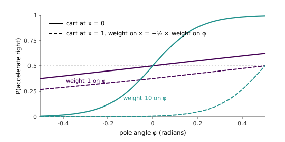
25:47 To see that this can express sensible behaviour, take . Then , and the probability of accelerating right is : the further the pole leans to the right, the likelier the cart is to accelerate right and get back under it. This ignores where the cart is, and a cart that keeps chasing the pole will run off the end of its track. 27:18 With the position enters with a negative weight, so the further right the cart already is, the less likely it is to accelerate further right. The general problem is to find the five numbers that trade off position, velocity, angle and angular velocity best, and that is what the algorithm will do.
Figure 20.1 plots these policies. One thing the board example hides is scale. With a weight of 1 on an angle measured in radians, a pole tilted half a radian, nearly thirty degrees, still gets accelerated the right way only 62 % of the time: the policy is close to a coin flip over every angle a balancing controller would see. The signs in say which way to lean; the magnitude says how decisively, and a weight of 10 turns the same policy into almost a step. The learning algorithm has to find both.
figures/20-policy-search/make_diagrams.py.
49:04 Later, answering a question, Ng gives the reason for the switch to stochastic policies. A deterministic policy over two actions is a step function of , either left or right, and there is no derivative to follow. Probabilities move smoothly with , so the expected payoff becomes differentiable and gradient ascent applies.
20.4 The objective
29:03 The goal is to choose to maximise the expected payoff when the policy is run:
in the finite-horizon setting of Section 19.2, with rewards that may depend on the action as in Section 19.1. For the pendulum the reward might be whenever the pole falls over and 0 otherwise.
30:15 One difference from value iteration is easy to miss. gives the optimal policy for every starting state at once, so a single is simultaneously best from wherever the system begins. Policy search optimises from one fixed initial state , or one fixed distribution over initial states, and the policy it finds is best for that start. A policy class too small to contain forces a trade-off between states, and the initial distribution decides which states the trade-off favours.
20.5 REINFORCE
32:02 To keep the board manageable, Ng sets : two states and two actions. The expectation in Equation 20.2 is then a sum over every state-action sequence, weighted by its probability:
The initial distribution and the transition probabilities do not depend on ; only the two policy factors do. Everything below carries over to longer horizons with longer products and sums.
34:58 The algorithm that climbs this objective is called REINFORCE, after Williams’ 1992 paper (Simple statistical gradient-following algorithms for connectionist reinforcement learning). Ng presents its core and notes that the original has a few further refinements, one of which comes up below. Each iteration does three things:
- Run the system for steps under the current policy, sampling each action from , to get a sequence .
- Compute the payoff, the sum of the rewards along it.
- Update
37:48 Each update is random, because it depends on which states the system happened to visit and which actions the policy happened to draw. Ng’s picture is the one he drew for stochastic gradient descent on linear regression (Section 2.6): batch gradient descent heads straight for the optimum, while the stochastic version takes a jittery path that heads the right way on average. The claim is that REINFORCE is stochastic gradient ascent on the expected payoff: the expected value of the bracketed update is exactly the gradient of Equation 20.3.
20.6 Why the update follows the gradient
40:05 The proof is three lines of calculus. Differentiate Equation 20.3. Inside the sum only the two factors depend on , so the product rule gives two terms:
43:58 Now multiply and divide the first term by and the second by . Both terms then contain the full product , which is the probability of the whole sequence, and it factors out:
That is a probability-weighted sum over sequences of exactly the quantity REINFORCE adds to in Equation 20.4, so it is the expected value of that update. 48:03 With a small learning rate, many updates average out and the parameters drift along the gradient of the expected payoff. Each ratio is , the score of the action, which is the form the update is usually written in today. For the logistic policy Equation 20.1 it is the familiar , the same expression as the logistic-regression gradient (Section 3.6), now weighted by the payoff instead of the label error.
The generator for this chapter checks Equation 20.5 by two routes on a small pole-balancing problem described below. It enumerates every two-step trajectory to compute the expected REINFORCE update exactly, differentiates the expected payoff numerically through a dynamic programme, and finds the two agree to at twenty random settings of .
48:36 A student asks whether the derivation depends on the logistic form. It does not. Nothing in it used anything about except that it is the probability of the action and that it is differentiable in . A softmax over many actions works, and so does a logistic function of elaborate features of the state. 50:48 The same holds for continuous actions, which policy search handles without discretizing. If the action is a real number, the force on the cart or a car’s steering angle, a natural policy is with Gaussian ; becomes a Gaussian density, and the same update applies with the density in place of the probability.
49:40 Another student asks why not skip all this and train the helicopter by supervised learning on a human pilot’s stick inputs, learning the map from state to the pilot’s action. Ng thinks that might fly a helicopter slowly without crashing it, but not well. Learning from rewards is what let the controller fly some manoeuvres better than the human pilots did, and imitation gives the controller no signal for doing better than the teacher it copies.
20.7 Why REINFORCE is slow, and what helps
58:14 Ng is blunt about the cost. The expected update is exactly right, but each individual update is very noisy, so REINFORCE needs a small learning rate and a very large number of iterations. Papers that use it routinely report millions of them.
Part of that noise is self-inflicted, and the lecture’s form of the update shows where. Equation 20.4 multiplies the score of every action by the whole payoff, including rewards collected before the action was taken. The action at step cannot have affected those, and the corresponding terms average to zero. The reason is an identity that holds in every state:
A reward from before step is fixed by the time is drawn, so its product with the score of has mean zero. Those terms contribute nothing to the expected update and add variance to every individual one. Dropping them gives the update usually written for REINFORCE, with each action weighted only by the rewards that follow it:
The same identity licenses , a baseline: any quantity that does not depend on the action can be subtracted from the weight without changing the expected update. A good choice is the expected reward-to-go from step , which turns the weight into a measure of whether the run went better or worse than usual from that point. That is one of the refinements in Williams’ original algorithm, whose update is written with a reinforcement baseline from the start.
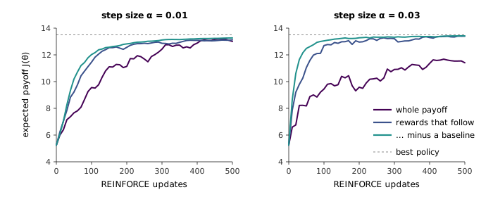
The generator checks all three versions on a toy that keeps every expectation computable. The pole’s tilt is an integer from to , and it falls, ending the reward, if it leaves that range. Gravity pushes a tilted pole further over with probability one half; an upright pole wobbles either way with probability a quarter each. Accelerating corrects the tilt by one step with probability 0.6. The reward is 1 for every step the pole is up, over 20 transitions, and the policy is . At , the coin-flip policy, the expected payoff is 5.25 and the best deterministic policy gets 13.50. Averaged over 20,000 runs, all three estimators agree with the numerically differentiated gradient, , within their standard errors. Their variances do not agree. On , the lecture’s version has variance 174, the rewards-that-follow version 51, and with the baseline 19: nine times less noise for the same expected step.
figures/20-policy-search/make_diagrams.py.
Figure 20.2 shows what that buys. At step size all three approach the optimum, but the lecture’s version needs about 290 updates for its average run to reach 90 % of the best payoff, against 130 and 110 for the other two. At the lower-variance versions get there in about 100 and 40 updates. The lecture’s version does not get there at all on average: after 500 updates, 5 of its 20 runs are still below 90 % of the best payoff. Inspecting them shows how it fails. A single large, noisy step throws the intercept far from zero, the policy then pushes the same way in almost every state, and with the sigmoid saturated the scores, and so the further updates, are tiny. A larger step size is not available to an estimator this noisy, which is Ng’s point about small learning rates, and removing terms that average to zero is the cheapest way to make it available.
20.8 Partial observability
52:24 Ng names two situations in which direct policy search is the better choice. The first is a partially observable MDP, or POMDP. Suppose the pendulum has a position sensor and an angle sensor but nothing that measures velocities, and both sensors are noisy. On each step the agent sees not the state but an observation
two noisy readings of four state variables, and it still has to choose an action.
Value-function methods are stuck here. 55:34 Even with and in hand, the policy needs the state, which the agent does not have. There is a large academic literature that extends value-based methods to POMDPs, but in Ng’s assessment those algorithms are very complicated and are not widely used in production. Policy search needs no extension. Define the policy on what the agent can see,
and REINFORCE runs unchanged: nothing in Equation 20.5 required the policy’s input to be the state, only that the action’s probability be a differentiable function of . The policy may not be as good as one that sees the state, but the algorithm finds the best one of this form.
57:00 The input can be any features of the history, not just the current reading. A common design is to run a state estimator, such as a Kalman filter, over all the measurements so far, which produces an estimate of the full state vector including the velocities, and feed that estimate to the policy as its features.
20.9 Policy or value function?
58:59 The second consideration is which object is simpler. Ng distinguishes low-level control tasks, the ones a skilled human does by feel with a joystick in a fraction of a second: hovering a helicopter, balancing an inverted pendulum, keeping a car in its lane on a straight road. For those a simple function of the state, often close to linear, is a good policy, so a small policy class contains a good answer, and direct policy search is promising. Chess and Go are the opposite: a good move depends on reasoning several steps ahead, no simple function of the board position plays well, and value-function approximation is the more promising route. Driving sits on both sides. Staying in the lane is low-level control; planning to overtake one car before a truck arrives in that lane is multi-step reasoning.
1:02:01 The helicopter went through both phases. Ng’s first controllers, including the one in the inverted-flight video at the start of the lecture, came from a direct policy search algorithm, a relative of REINFORCE rather than REINFORCE itself. More complicated manoeuvres called for methods closer to value-function approximation. The two families combine, too: Ng cites AlphaGo, which trained a policy network and a value network and used both in its search.
1:03:20 The course closes with where reinforcement learning was being applied in 2018. Game playing is the visible case, but Ng expects robotics to matter most, and mentions large-machine control in industry, factory optimisation, sequential medical decisions in which each test result decides the next step, and the execution of large stock trades in pieces small enough not to move the price. The common thread is the one the whole reinforcement-learning unit has been about: a sequence of decisions whose payoff arrives only over time.
The 2018 notes for this part of the course, cs229-notes12, cover MDPs, value and policy iteration and continuous-state MDPs, and end before policy search. The lecture is the source for REINFORCE here; Williams’ 1992 paper has the general form, including the baseline.