17 MDPs and Value/Policy Iteration
Lecture 17
Bellman equation, value iteration, policy iteration, Markov decision processes, exploration versus exploitation
Lecture video: Lecture 17: MDPs and Value/Policy Iteration · 1:19:14
Based on the lecture by Andrew Ng — CS229, Stanford University, Autumn 2018.
Lecture 16 defined a Markov decision process and claimed an optimal policy for the 11-state gridworld without saying where it came from. This lecture supplies the method. It defines three objects: , the value of following a fixed policy; , the best value any policy can achieve; and , the policy that achieves it. Each satisfies a version of Bellman’s equation, and the two standard algorithms, value iteration and policy iteration, are two ways of solving those equations. The lecture then drops the assumption that the transition probabilities are known. It estimates them from the robot’s own experience, and this raises the question of how much the robot should explore.
17.1 The value of a policy
6:46 For a policy , the value function gives the expected total payoff of starting in and following for ever:
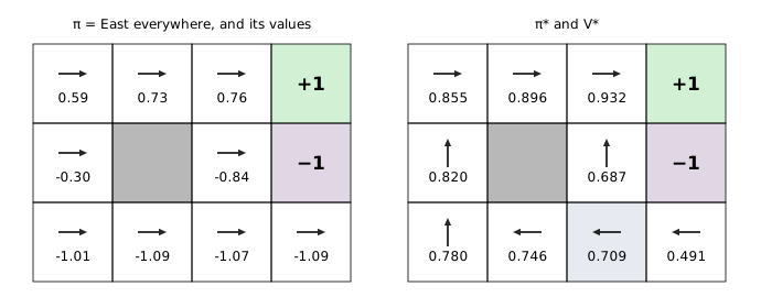
8:40 Ng’s example is deliberately poor. From some states it drives straight for the . The left half of Figure 17.1 uses a concrete policy of that kind, East from every state. On the top row it reaches the and is worth about 0.6 to 0.76. Along the middle and bottom rows it runs into the , or stalls against the east wall paying a step, and is worth about to . The cells are absorbing: once the robot reaches one, it collects that reward and the world ends.
10:57 The equation that governs comes from splitting the payoff after its first term. Factor one out of everything after :
The bracket is the payoff of a robot that starts in and follows . Its expectation is , and is drawn from , because in state the policy takes action . Writing for the next state gives Bellman’s equation for :
The first term is the immediate reward, which the robot gets just for waking up in . The second is the discounted expected future reward.
19:42 For a fixed , Equation 17.1 is linear in the unknowns . For , with going North, it reads
and one such equation for each of the 11 states gives 11 linear equations in 11 unknowns. A linear solver handles that instantly. The generator solves the system for the East policy and checks the result against 5,000 sweeps of repeated substitution into Equation 17.1. The two agree to .
17.2 The optimal value function and the optimal policy
24:47 The optimal value function is the best value any policy achieves from each state:
Ng flags a terminology trap. Both and are called “value functions”, but one belongs to a particular policy, good or bad, and the other to the best of them. The maximum is over a combinatorially large set, policies even for this small grid, so the definition does not suggest how to compute . Its Bellman equation does.
27:12 Run the same argument as for Equation 17.1, but let the robot choose its first action well. It collects for waking up in . Whatever action it takes, it then lands in and can collect at most from there. The best first action is the one with the largest expected continuation, so
29:44 If were known, the optimal action would be the one that attains that maximum. Ng asks the room what to do in state , and the answer is already in Equation 17.2:
is dropped because a positive constant does not move an argmax. 32:50 Ng states, without proof, that this policy is optimal from every state at once: for every and every . One policy is best everywhere, so no state has to trade off against another. The generator checks both halves. The value of the greedy policy, solved from its own linear system, equals to , and is at least , state by state, for 3,000 random policies. The plan is therefore to find and then read off with Equation 17.3.
17.3 Value iteration
35:22 Value iteration treats Equation 17.2 as an update rule:
- Initialise for every .
- Repeat until convergence: for every , .
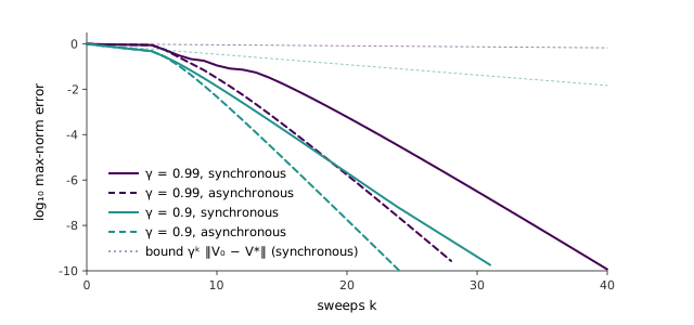
38:07 There are two ways to carry out step 2, and Ng compares them to gradient descent. A synchronous update computes the right-hand side for all 11 states from the old values, then overwrites all 11 at once. In vector form this is , where is called the Bellman backup operator. An asynchronous update sweeps through the states one at a time and overwrites each value as soon as it is computed, so later states in the sweep already use the new values. Both converge to .
Ng’s default is the synchronous form, because it is a matrix operation and vectorises. He says “asynchronous” at this point in the recording, but the reason he gives, vectorisation, and the procedure he describes, compute all eleven and then update, are the synchronous one. The asynchronous form has the opposite advantage: it needs fewer sweeps. On the gridworld with , the max-norm error falls below after 21 asynchronous sweeps against 29 synchronous ones (Figure 17.2).
40:32 A student asks how to code the absorbing states. One way is to give them transition probabilities of zero to every state, so that their value is just . Another is to add a twelfth, zero-reward “sink” state that they lead to and that loops on itself. Ng calls the second cleaner and the first more common. Both give the same values.
43:07 Why does it converge? The problem set shows that is a contraction in the max norm: . Since , each synchronous sweep shrinks the error by at least a factor , so . Ng turns this into a rule of thumb: at , value iteration needs a few hundred iterations, and at a few dozen.
The bound is right but, for this MDP, very loose. Taken literally, it needs 1,375 sweeps per unit of initial error to reach at , and 132 at . The gridworld gets there in 29 sweeps at and 21 at . The generator asserts that every synchronous sweep is within the bound, so nothing here contradicts the theorem. The reason is the absorbing states. After sweeps the remaining error is roughly the discounted value of what happens beyond step . Under , starting from , the robot is still wandering after 10 steps with probability 0.04, and after 20 steps with probability essentially zero, so there is little left to discount. The factor only governs the rate when the process can run on for a long time without ending. The more useful fact for practice is that the policy converges before the values. With , the greedy policy Equation 17.3 of the synchronous estimate is already exactly after 11 sweeps, while the values are still off by as much as 0.08.
17.4 Reading the policy off
45:15 Ng writes the converged on the board and uses it to justify the West arrow at that lecture 16 asserted. Going West reaches with probability 0.8, where . It slips North to , worth 0.69, with probability 0.1, and South into the wall, staying at , worth 0.71, with probability 0.1. The expected value is 0.740. Going North gives , so West wins.
The generator’s (Figure 17.1, right) matches the board values to two decimals: 0.746, 0.687, 0.709 and 0.491. Computed from the unrounded values, the two expectations are 0.736 and 0.674. Ng adds that a full check compares all four actions, and the full check is instructive. South, at 0.691, beats North: bumping into the wall and staying put is the second-best action, because North risks the slip into . East is last at 0.532.
17.5 Policy iteration
50:18 Policy iteration keeps a policy, not a value function, at the centre:
- Initialise randomly.
- Repeat until stops changing:
- , by solving the linear system Equation 17.1;
- for every , .
Step (b) pretends that the current is optimal and acts greedily on it. Value iteration waits until has converged to extract a policy. Policy iteration extracts a new one on every round. 54:44 The trade-off, as Ng puts it, is the linear solve in step (a). For 11 states, or a few hundred, it is trivial, and policy iteration is fast. For 10,000 states or a million, solving the system on every round is expensive, and he would use value iteration. He also notes a more academic difference. Value iteration approaches and never exactly reaches it, as gradient descent approaches the minimum of a least-squares cost. Policy iteration stops after a finite number of rounds, at exactly and exactly , the way the normal equations jump straight to the answer. It must stop, because each round improves the policy, by the policy improvement theorem, and there are only finitely many policies to improve through.
The generator checks this on the gridworld. Started from 200 random policies, policy iteration needs between 2 and 8 evaluations, 5 on average, and always ends at the of Figure 17.1. From “always East” it needs 3. The values never decrease from one round to the next, in any state. In practice, Ng says, he sees value iteration used more, because real problems are large. For small ones policy iteration may converge a little faster.
Both algorithms, the synchronous and asynchronous variants, and the statement that policy iteration terminates are in cs229-notes12, section 2. The contraction argument for value iteration is a homework problem in the course.
17.6 Learning the model
58:41 So far has been given. For a real robot, a helicopter or a chess opponent, it usually is not, and has to be estimated from experience. Run some policy for a while, count what happens, and use the maximum-likelihood estimate
When the denominator is zero, because has never been tried in , the common heuristic is a uniform guess, .
1:01:41 Laplace smoothing would also avoid the : add 1 to every numerator and to every denominator. Ng says it is allowed but uncommon, because, unlike naive Bayes, MDP solvers are not badly hurt by zero estimates. The generator suggests a stronger statement: on the gridworld, smoothing makes things worse. It runs a uniformly random policy for a given number of moves, builds with and without smoothing, solves for the policy, and scores it by its true loss, the largest over states, averaged over 40 runs. The plain counts lose 0.078 after 1,000 moves and 0.010 after 10,000. With smoothing the losses are 0.263 and 0.023. The reason is visible in the formula. Smoothing gives every action a small probability of moving the robot to every state, including straight to the or from across the grid. With 11 states and only a few visits per state-action pair, that invented mass is large, and it is exactly the mass the optimal policy is most sensitive to. Exact recovery of is rare either way, 14 runs in 40 even after 10,000 moves without smoothing, because of the 0.0005 margin at noted in lecture 16. Measuring the loss, not whether the policy is exactly , is the fair test.
1:03:01 Put together, the practical loop is:
- Take actions according to some policy to gain experience in the MDP.
- Update the estimates of from the counts, and of if it is unknown.
- Solve Bellman’s equations for the estimated MDP by value iteration, warm-started from the previous if convenient, to get a new .
- Update to be greedy with respect to , and repeat.
1:06:03 The reward is usually part of the problem specification, but not always. For a trading application the reward is a day’s return, and for a car it might be a penalty for every pothole. Both are random functions of the state, so the same loop estimates the expected reward of each state by averaging what it observes.
17.7 Exploration versus exploitation
1:07:33 The loop above is greedy: it always acts on its current best estimate. Ng shows the trouble with a different MDP. A robot starts with a nearby and a farther away. If its first runs happen to reach the , the estimated model says that going there works, and the greedy policy keeps going there. Every trip ends at the , so the robot’s experience stays in that half of the state space, and the is never found. Acting on what is known is exploitation. Trying actions that look worse to learn something new is exploration. The tension between them is not academic. Ng’s example is online advertising. Showing only the ads a user is predicted to click maximises short-term revenue. Showing occasional others is how the platform discovers interests nobody knew the user had.
1:13:28 The standard fix is ε-greedy exploration. On each step, with probability take the action , and with probability , for instance 0.1, take a random one. Ng points out that the name is backwards, since is the probability of acting randomly, not greedily, but it is the name everyone uses. With every action keeps being tried in every state the robot can reach, so the estimated model converges to the true one and the planned policy to , though finding a remote reward by chance can take a long time.
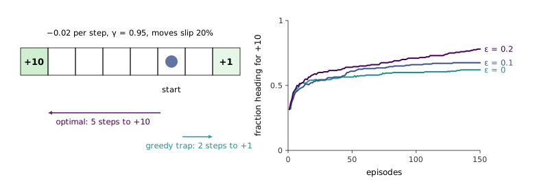
Figure 17.3 makes Ng’s example concrete in one dimension, in a toy of our own: an eight-cell corridor with the five steps to the left of the start and the two steps to the right. Moves slip 20% of the time, each step costs 0.02, , and the robot learns both and as above. Going left is worth about 7.65 and going right 0.86, so the right answer is not close. Over 200 independent learners, the fraction whose policy heads for the after 150 episodes is 0.62 for the greedy learner, 0.68 with and 0.78 with . Two details are worth noticing. The greedy learner is not completely stuck: its curve keeps creeping up, presumably because slipping moves sometimes carry it left without being asked. And none of the curves has reached 1, which is Ng’s caveat about how long a remote reward can take to find.
1:16:17 Asked whether should stay fixed, Ng says there are many heuristics, and a reasonable one is to start large and shrink it. Another is Boltzmann exploration. Instead of a uniformly random action with probability , choose action with probability proportional to , where is the estimated value of taking and is a temperature. Actions that look nearly as good as the best are tried often, and actions that look terrible almost never. A student asks about rewarding the robot for visiting states it has never seen. That is intrinsic motivation, a research line Ng suggests looking up. And asked how often to re-plan, he says as often as the computation allows. It does no harm. With a physical robot or helicopter, where each flight is a session, re-planning between flights is the natural rhythm.
Estimating and from experience, with the rule for untried actions and the warm-started value iteration loop, is in cs229-notes12, section 3. The notes do not treat exploration. Lecture 18 extends the framework to continuous states, covered in section 4 of the same notes.