16 Independent Component Analysis and RL
Lecture 16
independent component analysis, cocktail party problem, reinforcement learning, Markov decision processes, discount factor
Lecture video: Lecture 16: Independent Component Analysis and RL · 1:18:10
Based on the lecture by Andrew Ng — CS229, Stanford University, Autumn 2018.
The lecture has two halves that share nothing but a date. The first finishes independent components analysis. Chapter 15 set up the cocktail-party model and showed that the sources can be recovered only up to order, sign and scale. This chapter adds the reason ICA needs non-Gaussian sources, writes down the likelihood of the unmixing matrix , and derives the stochastic gradient rule that maximises it. The second half opens the last part of the course, reinforcement learning. It introduces the Markov decision process and the 11-state gridworld that lectures 16 and 17 use as their running example, and states the goal: a policy that maximises the expected discounted sum of rewards.
16.1 Gaussian sources cannot be unmixed
3:07 Chapter 15’s picture of why ICA works used sources uniform on . Their joint distribution fills a square, the mixing matrix shears it into a parallelogram, and the corners of the parallelogram give away the directions of the original axes. Ng now asks what happens if the sources are Gaussian instead. Two independent standard Gaussians have a joint density with circular contours. A mixing matrix stretches the circle into an ellipse, and an unmixing matrix that maps the ellipse back to a circle is easy to find. But it is not unique, because every rotation of a circle is the same circle. If turns the data back into independent unit Gaussians, so does for any rotation , and nothing in the data can choose between them.
The official notes make this precise. If then is Gaussian with covariance , and for any orthogonal the mixing matrix gives with covariance . The two models produce the same distribution of recordings. The generator checks the same fact from the other side: with a Gaussian source prior, the log-likelihood of the 1,500-example dataset used below is unchanged, to rounding error, when the true unmixing matrix is rotated by 10°, 30°, 45° or 60°. Under the logistic prior introduced below it drops by 0.030 per example at 45°, so that likelihood does single out the right rotation.
6:44 Ng cites the theorem behind this informally: the Gaussian is the only distribution of independent components that is rotationally symmetric, and so ICA is possible exactly when the data are non-Gaussian. The careful version, due to Comon, is slightly weaker in its demand: the sources are identifiable up to order and scale as long as at most one of them is Gaussian. One Gaussian source has no other Gaussian to be confused with, and two or more can be rotated into one another.
16.2 The density of a linear transformation
12:08 To fit by maximum likelihood we need , the density of the recordings, given , the density of the sources, and the relation . The tempting answer is . Since is invertible, every corresponds to exactly one , so it seems the probability of seeing is the probability of the matching . Ng points out that this is correct for probability mass functions and wrong for densities.
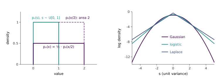
14:31 His one-dimensional example shows why. Let be uniform on , so there, and let , so and . Then is uniform on , and a density spread over twice the width must be half as tall: on . The naive formula gives on , which integrates to 2 (Figure 16.1, left). The missing factor is the determinant:
where is the absolute value of the determinant of . In one dimension it is just , and the generator confirms numerically that the corrected density integrates to 1 and the naive one to 2. The intuition carries to dimensions. maps the unit cube of source space to a parallelepiped of volume , so probability spread over that volume has its density divided by , that is, multiplied by .
16.3 A prior for the sources: the sigmoid as a CDF
18:22 The last modelling choice is , the density of a single speaker’s signal. It must not be Gaussian. Ng specifies it through its cumulative distribution function , which rises smoothly from 0 to 1, and recovers the density as . The question then becomes which familiar function rises smoothly from 0 to 1, and the sigmoid is the obvious answer. So the model takes , with , and
This is the logistic density. Ng’s argument for it is its tails. A Gaussian density falls like ; the logistic falls like , so large values are far more likely, and that, he says, describes recorded speech and many natural signals better. The right panel of Figure 16.1 shows the difference on a log scale. At equal variance, the logistic density at four standard deviations is 9.6 times the Gaussian’s, and its excess kurtosis is 1.2 where the Gaussian’s is 0. Ng adds that a two-sided exponential, the Laplace density, works as well, and he has used it himself. Its tails are heavier still, with excess kurtosis 3. The sigmoid, he recalls, was simply the choice that early ICA researchers needed and tried, in Bell and Sejnowski’s information-maximisation algorithm, and it has stayed the default because it works.
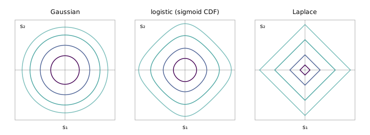
28:24 A student asks why the joint density of two logistic sources is not also rotationally symmetric. Ng sketches the contours of a Laplace pair as diamonds and guesses that the logistic looks “a bit like that too”, inviting the class to plot it. The plot is Figure 16.2, and the guess is half right. Close to the origin the logistic density is nearly Gaussian, because for small , so the inner contours are almost circles: along the diagonal the innermost one reaches 0.98 of its distance along an axis. Farther out the linear tails take over and the contours become diamonds, with that ratio falling to 0.86 at the outermost level drawn. A Laplace pair has diamonds at every level, with ratio , and a Gaussian pair has circles. What matters for ICA is only that the logistic contours are not circles. Any departure from rotational symmetry gives the likelihood a preferred orientation.
16.4 Maximum likelihood for the unmixing matrix
21:39 With these pieces the likelihood is short. ICA’s central assumption is that the speakers are independent, so the joint source density is a product, . Combining that with Equation 16.1 and , where is the -th row of , gives
For a training set , one microphone reading per instant, the log-likelihood of is
26:02 Ng writes the derivative without deriving it. The official notes do the algebra, which needs the identity . For one example it gives the stochastic gradient ascent rule
The first term comes from the prior: . The second comes from the determinant and keeps from collapsing to zero, which would otherwise make every zero and every source density maximal. A student catches a slip on the board here: the bracket should hold , with the sigmoid. The generator compares the analytic gradient with central finite differences of Equation 16.2, and they agree to .
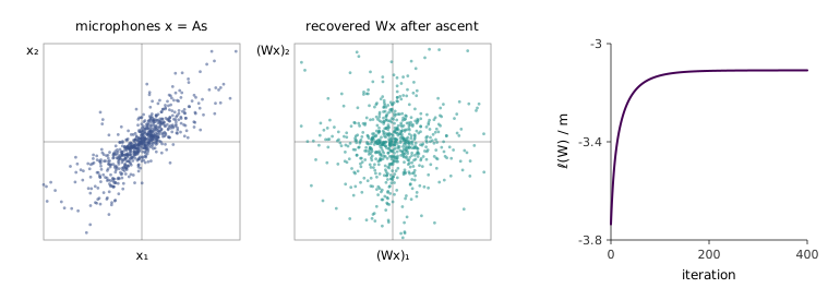
27:12 The whole algorithm, then, is to initialise , run gradient ascent on Equation 16.2, and read each source off as . Playing through a speaker plays back speaker 1. Figure 16.3 runs it on 1,500 readings of two independent Laplace sources mixed by a fixed . Batch gradient ascent from raises the average log-likelihood from to and levels off. The product it ends with is , a scaled identity up to cross-talk of under 4%, and each recovered signal correlates with its source at 0.999 or above. The scale is not 1, because maximum likelihood rescales each source to suit the logistic prior. That is the scale ambiguity from chapter 15, resolved arbitrarily. The data here are generated exactly by the ICA model. Ng’s real-room recording separated less cleanly, for the reasons Section 15.8 gives.
The density of a linear transformation and the full derivation of Equation 16.3 are in cs229-notes11, sections 2 and 3. The notes also remark that the data should have zero mean, which the sigmoid prior assumes, and that the training examples, being successive moments of audio, are not independent. The notes say this does not hurt the result, and that visiting the examples in a random order can speed up stochastic gradient ascent.
16.5 Where ICA is used, and where it breaks
30:03 Asked for the closest nonlinear extension of ICA, Ng says there is no good answer yet and points to his own group’s work on stacking it. The large unsupervised network that learned to detect faces and cats in YouTube frames (Le et al., 2012) was trained layer by layer with an objective the paper calls reconstruction topographic ICA, a close relative of sparse coding. Ng’s view is that hierarchical versions of ICA and sparse coding lost attention when supervised deep learning took off, and deserve more of it than they get.
33:46 The standard application is cleaning electroencephalography (EEG) data. Electrodes on the scalp each record a weighted sum of the electrical activity of many brain processes at once: the heartbeat, eye blinks, everything else. That is a cocktail party in the head, and ICA unmixes it the same way. An analyst identifies the components that are heartbeat or blink artefacts, removes them, and remixes the rest (Jung et al., 2000). The clean signal is then the input to whatever comes next, such as a classifier that tries to tell from EEG whether a person is thinking of a person or an object. Run on small patches of natural images, ICA finds components that are localised, oriented edges (Bell and Sejnowski, 1997). The same result from sparse coding (Olshausen and Field, 1996) is one of the reasons neuroscientists ask whether the visual cortex learns its edge detectors this way.
40:41 A student had asked whether the number of microphones must equal the number of speakers. Ng’s answer is that more microphones than speakers is fine: run ICA, perhaps slightly modified, and some of the recovered sources come out silent. Fewer microphones than speakers is a research problem. With one microphone and two speakers, is and cannot be inverted, so separation needs knowledge beyond independence. A low voice and a high voice can sometimes be pulled apart, two similar voices hardly at all.
The “slightly modified” matters more than it sounds. Run Equation 16.2 unchanged with ten microphones and five speakers, and is while the recordings fill only a five-dimensional subspace. Any row orthogonal to that subspace outputs exactly zero for every example, so it is one of the silent sources. Scaling that row by leaves its terms unchanged and multiplies by . The log-likelihood therefore grows by without bound. The generator confirms the exact gain for three microphones and two sources. So the silent sources are where the plain algorithm diverges, not a harmless by-product. The usual modification is to reduce the recordings to as many dimensions as there are sources, with PCA, before running ICA.
Ng’s other suggestion, from a student’s follow-up, is to parameterise the model by the rectangular mixing matrix , here, instead of . That avoids the problem but loses the convenient formula Equation 16.1, which needs a square . How many sources to assume, he says, is like choosing in k-means: try several and look for components that come out near-silent.
16.6 Why reinforcement learning
49:52 The fourth and last part of the course is reinforcement learning. Ng motivates it with the autonomous helicopter from lecture 1. At every moment the helicopter is in some state, its position, orientation and velocity, and must choose how to move the control sticks. Supervised learning would need, for each state, the one correct stick position, and nobody can write that down. What a designer can write is a reward function: high when the helicopter flies the intended trajectory, very negative when it crashes. Ng compares it to training a dog. You cannot tell the dog what to do, but you can say “good dog” and “bad dog”, and it learns to do more of what earns the first. Games fit the same mould. Nobody knows the one best chess move in a given position, but a program can play and be rewarded with for a win, for a loss and 0 for a draw.
53:41 Such sparse feedback creates what Ng calls the credit assignment problem. A chess program checkmated on move 50 receives , but the losing blunder may have been on move 20, with the remaining 30 moves only playing out a lost position. A self-driving car that crashes usually made the decisive mistake seconds earlier, not at the instant of impact. Given only the final reward, the algorithm has to work out which of its earlier actions to do more of and which to do less of. Every algorithm in the rest of the course solves this problem, at least indirectly, and the value functions of lecture 17 are the main way they do it.
16.7 Markov decision processes
56:29 Reinforcement learning problems are modelled as Markov decision processes. An MDP is a five-tuple :
- , the set of states: chess positions, or the helicopter’s possible positions, orientations and velocities;
- , the set of actions: legal moves, or stick positions;
- , the state transition probabilities: for each state and action , a distribution over the next state;
- , the discount factor, explained in Section 16.8;
- , the reward function.
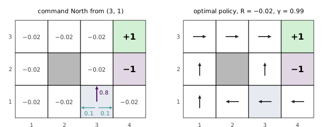
58:29 The running example is small enough to draw. Ng takes it from Russell and Norvig’s textbook (Figure 16.4). A robot moves on a grid with one cell blocked by a pillar, so there are 11 states, written from the bottom left. The actions are the four compass directions. Real robots’ wheels slip, so the model makes moves noisy. A command goes in the intended direction with probability 0.8 and veers to each side with probability 0.1. From , a command to go North reaches with probability 0.8, with 0.1 and with 0.1. A move into a wall or the pillar leaves the robot where it is. Ng stresses that this is a caricature of real robot dynamics, chosen so that the whole MDP fits on the board.
1:02:41 The task is specified entirely through the reward. Ng puts at , the goal, and at , a cell to avoid. To make the robot hurry, every other state carries a small negative reward, , which Ng describes as charging the robot for the electricity it spends loitering. Lecture 17 adds that the cells are absorbing: once the robot reaches one, it collects that reward and the world ends.
16.8 Payoff, discounting and policies
1:05:15 The robot wakes in some state and chooses an action . The world moves it to , it chooses , moves to , and so on. Its total payoff is the discounted sum of the rewards along the way:
The goal is to choose actions that maximise the expected total payoff, since the transitions are random. With around 0.99, a reward one step from now counts 0.99 as much as one now, and one a hundred steps away about 0.37 as much.
1:08:00 Ng gives two reasons for , and says plainly that the second is the real one. The first is the time value of money. A dollar today is worth more than a dollar next year, because it can earn interest, and by the same logic a payment is better postponed than made now. So makes the robot hurry towards positive rewards and put off negative ones. The second is that with the algorithms provably converge, and with many of them do not, or are much harder to analyse. A student supplies the mechanism. Without discounting, the sum Equation 16.4 can grow or shrink without bound. With it, . For a robot that loiters for ever at per step with , that is , a finite number an algorithm can reason about.
1:11:28 What a reinforcement learning algorithm produces is a policy, , a rule for which action to take in each state. Executing means taking in whatever state the robot is in. Ng shows the optimal policy for the gridworld (Figure 16.4, right), computed offline. Lecture 17 derives value iteration, the algorithm that computes it. The generator runs it and reproduces, to two decimals, the values Ng later reads off the board.
1:14:44 The interesting cell is . North is the direct route: two steps to , then one East to the goal. But at a 0.1 chance of slipping East lands the robot on . West goes all the way round by and the top row, which costs more steps and more discounting, but never passes the . Ng’s point is that the answer is not obvious by eye, and the optimal policy takes the long, safe route. The generator measures how fine the distinction is. At , the expected value of the next state is 0.736 for West against 0.674 for North, and the runner-up is not North but South, at 0.691: bumping into the wall and staying put is better than going North. The choice holds only while the step reward lies between 0 and . Below that, loitering costs enough that the risky short route wins. Elsewhere the margins are smaller still. At , North beats West by 0.0005, and only because the step reward is below ; at , West beats South by 0.003. An MDP solver makes these distinctions exactly. A person eyeballing the grid would not.
1:16:13 Two last questions point ahead. Chess fits the framework if a “state” is the board when it is your turn: you move, the opponent moves, and the opponent’s unknown reply becomes the randomness in . And the probabilities 0.8, 0.1, 0.1 need not be given. For a real robot they are usually estimated from data, which is how lecture 17 ends. The number of policies is finite but large. Lecture 17 counts it as , though only the nine non-absorbing states need an action, so . Enumerating them is hopeless for any realistic MDP, and the next lecture’s value and policy iteration avoid enumeration altogether.
Markov decision processes, the five-tuple, the total payoff and policies are in cs229-notes12, section 1. The notes allow rewards that depend on the action, , and mention finite-horizon MDPs. The lecture keeps to and infinite horizons.