Learning Theory
learning theory, empirical risk minimization, Hoeffding’s inequality, union bound, uniform convergence, VC dimension
Lecture video: Discussion Section: Learning Theory · 1:26:03
Based on the Friday discussion section of CS229, Stanford University, Autumn 2018, taught by a member of the course staff.
Lecture 8 told you to choose models on held-out data because training error is optimistic. This section asks how optimistic, and answers with a theorem: if an algorithm picks the hypothesis with the lowest training error from a class of hypotheses, then with probability at least its true error is within
of the best the class can do. Two facts are hiding in that expression. The number of examples needed grows only with the logarithm of the size of the class, and, once the class is infinite, the logarithm is replaced by a measure of the class’s expressiveness called the VC dimension. Getting there takes two elementary tools — the union bound and Hoeffding’s inequality — and a change of viewpoint about what a learning algorithm is.
Ng explained in lecture 8 that this material used to be part of the main lectures and moved to a Friday section because it matters less to making algorithms work than it once did. The section promises to state results rather than prove them, and the proofs are in cs229-notes4. What this chapter adds is the section’s own pictures, its answers to questions, and a computation behind every claim: the bounds are checked against exact probabilities and simulations, which also shows how loose they are.
The learning algorithm as an estimator
1:15 Everything rests on two assumptions. There is a fixed data distribution over pairs , from which both the training set and every future test example are drawn; and the examples are drawn independently. Without the first, training data say nothing about test data, and the theory has nothing to work with. Lecture 8’s aside about training on phone recordings to deploy on a smart speaker is exactly a case where it fails.
3:15 A learning algorithm is then a box. In goes a training set of samples from ; out comes a hypothesis , or equivalently, for a parametric class such as logistic regression in dimensions, a parameter vector . 4:43 The point the section makes first is that is random, the box is a deterministic function, and so its output is random too. Run the box on a different sample from and you get a different . In statistics the box is called an estimator, and the distribution of over repeated draws of is its sampling distribution.
6:22 Against this randomness stands a fixed target, a true parameter (or true hypothesis ) that we would like the box to output. It is unknown, but it is not random: there is no distribution over it. That is the frequentist stance of lecture 8, and the notation follows it — hats for things estimated from data, stars for the true values we never see. Asked whether must be a vector, the section answers that it can be anything we estimate, a scalar, a matrix, or a function with no parameters at all.
Bias and variance as moments of the sampling distribution
10:26 Lecture 8 pictured bias and variance in the data view: curves through points, underfitting and overfitting. The section redraws them in the parameter view, which makes them precise. Take a model with two parameters, so that each is a dot in the plane. Draw a training set of size , run the algorithm, plot the dot; draw another training set of the same size, plot another dot; repeat. The cloud of dots is a sample from the sampling distribution. 13:51 Bias asks whether the cloud is centred on : it is , a statement about the first moment. Variance asks how spread out the cloud is, the second moment. They are, in the section’s words, “just properties of the first and second moments of your sampling distribution”.
Figure 1 draws the clouds for two real estimators on one regression problem, with and two features correlated at — the situation of square footage and number of bedrooms. Least squares is unbiased, and at its cloud is centred on but enormous (total variance ), stretched along the direction in which correlated features cannot be told apart: raising while lowering barely changes the fit. Ridge regression with on the same training sets is pulled towards the origin, a bias of length , and its variance is thirty times smaller, . That is lecture 8’s claim that regularisation trades a little bias for a lot of variance, seen directly.
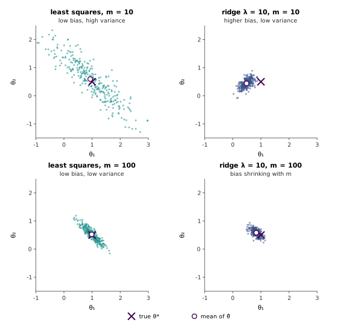
15:58 With ten times the data, every cloud tightens: least squares’ variance falls from to , roughly the factor of ten one expects from variance proportional to . As the variance goes to zero, and an estimator whose output converges to is called consistent. 17:56 An estimator with at every is called unbiased.
17:14 The rate at which variance falls with the section calls statistical efficiency, a measure of how well an algorithm squeezes information from data, and it offers as examples one algorithm whose variance falls like and another like . Those rates are not available to an unbiased estimator of a parameter in a regular model: the Cramér–Rao bound puts a floor of order under its variance. (Irregular models are different — the right endpoint of a uniform distribution can be estimated with variance of order — but the models in this course are regular.) What efficiency usually measures is the constant in front of . The mean and the median of a Gaussian sample are both unbiased estimates of its centre, both with variance proportional to ; but the median’s is larger by a factor of . The generator measures at for the mean and for the median at , against . Using the median wastes about a third of the data.
20:08 Informally, the section says, a high-bias algorithm is one that “no matter how much data or evidence you provide”, stays away from . That runs two ideas together, and the bottom row of Figure 1 separates them. Bias is defined at a fixed , as a student’s question prompts the section to confirm at 21:35; staying away forever is inconsistency. Ridge with a fixed is biased at every and yet consistent, because the penalty stays the same size while the data term grows in proportion to : its bias is at , at , at and at . 58:09 The same point answers a later question that the section leaves open, whether adding regularisation destroys the consistency of maximum likelihood. With a fixed penalty, it does not.
20:58 Bias and variance are separate properties; any combination of the two can occur. 22:18 High variance has two standard remedies. More data shrinks the cloud directly. Regularisation shrinks it by restricting where can go, usually at the price of moving its centre — which is the trade Figure 1 shows.
Approximation error and estimation error
25:02 The second picture is drawn in the space of all hypotheses. Somewhere in it is , the best possible hypothesis, with the lowest expected error under of any function whatsoever. 25:52 Our algorithm searches only a class — all logistic regression models, say, or all SVMs — drawn as a region that need not contain . 26:27 Inside the region is , the best hypothesis in the class. And what training on finite data actually produces is , a different point of for every training set.
27:51 For classification the error of a hypothesis is its probability of a mistake, and the training error is its frequency of mistakes on :
The first is called the generalisation error or risk; the second the empirical risk. 30:30 is the Bayes error, also called irreducible error: if the same can come with different labels, no function gets all of them right. Then the error of what we learn splits into three:
31:35 The identity is a telescoping sum, but each term names a different cause. Approximation error is the price of restricting ourselves to , a property of the class alone. 32:20 Estimation error is the price of having only examples, plus any quirks of the algorithm, and it shrinks as grows.
34:49 The section then says this decomposition and the bias–variance decomposition are related but not the same: estimation error itself splits into a variance part and a bias part, and “bias” in the usual sense is approximation error plus that estimation bias. For 0–1 loss this is a picture rather than an equation — there is no clean additive bias–variance identity for classification error — but for squared error it is exact, and worth seeing. Let , let be the average learned hypothesis, and measure error by . Then
and when is a linear space, such as all straight lines, is orthogonal to it, so Pythagoras splits the bias: , and the estimation error is the variance plus that same small term.
Figure 2 does this for straight lines fitted to eight points from a parabola, , with noise . The best line is flat, , and the approximation error is . The expected test error of the fitted line is , which splits as one way and the other. The difference between the two middle terms, , is the estimation bias: the average fitted line, , is not , because least squares on a misspecified model is biased at small . The generator asserts that both totals agree and that the Pythagorean identity holds.
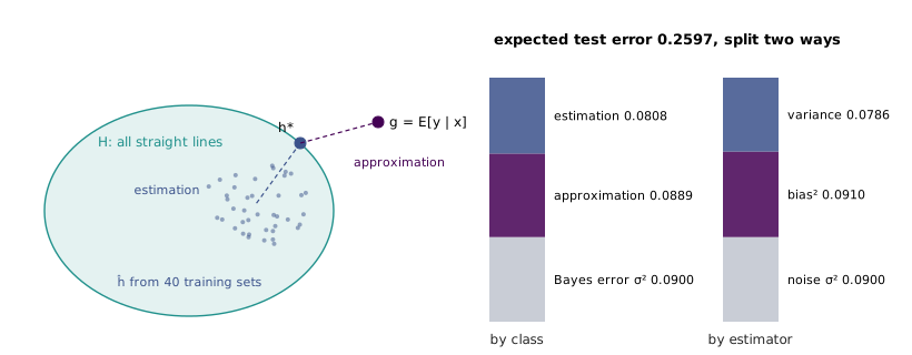
36:34 The picture also says how to fight each kind of error. To reduce bias, make bigger, so that it reaches closer to ; but a bigger class gives more room to wander, so variance tends to rise. 39:27 To reduce variance, make smaller — regularisation does this, by penalising hypotheses with large — and unless the shrinking happens to move towards , bias rises. 41:05 A student asks why not shrink the class towards ; because we do not know where is, and if we did there would be nothing to learn.
Empirical risk minimisation and two tools
44:56 Nothing so far depended on what happens inside the box. To prove something, the section now fixes the algorithm: empirical risk minimisation returns the hypothesis with the lowest training error,
47:36 This is “what we’ve been doing so far in the course”, with one honest caveat that the section mentions: logistic regression minimises the logistic loss, not the 0–1 training error of Equation 1, and SVMs minimise the hinge loss. Those losses are convex stand-ins for the count of mistakes, which is intractable to minimise directly. The theorems below are about the count of mistakes; they extend to the stand-ins with more work, which this section does not do.
49:25 Two questions organise the rest. How close is the training error of a hypothesis to its true error? And how close is the true error of the hypothesis ERM picks to that of the best in the class? 50:47 The first tool is the union bound: for any events , independent or not,
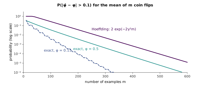
“If this looks trivial, it is trivial,” the section says. 52:00 The second is Hoeffding’s inequality, stated for the case needed here. Let be independent Bernoulli() variables and their mean. Then for any ,
The probability that an average of coin flips misses its expectation by more than a margin falls exponentially in the number of flips. The general version holds for any bounded independent variables, and the bound on the range is essential.
The bound is easy to check, because the exact probability is a binomial tail. Figure 3 compares them for . At the exact probabilities are for a fair coin and for , against a bound of . The bound holds at every and the generator tries, with the exact tail never more than of it. It has the right exponential rate, and it is loosest for coins far from fair, whose averages vary less — a looseness that matters here, because error rates of good classifiers are far from one half.
Uniform convergence for a finite class
59:54 The section’s central picture puts every hypothesis in on a horizontal axis and plots two curves above it: the true error , a fixed curve, and the training error , a random curve that changes with every training set. Figure 4 computes it for a class small enough that the true error of every member is a closed form. Inputs are uniform on , the label is flipped with probability , and contains ten threshold classifiers with . The Bayes error is . The class has no threshold at , so its best members, and , have error , an approximation error of .
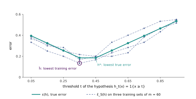
1:05:19 For one hypothesis fixed in advance, the training error is an average of independent Bernoulli variables whose mean is , so Hoeffding applies directly:
On average over training sets the dashed curve passes through the solid one at every , and with more data it hugs it more tightly. 1:08:16 But this is useless as it stands, and the section is precise about why: ERM does not fix in advance. It looks at the training set and picks the hypothesis whose dashed curve is lowest, so depends on and its training error is no longer an unbiased average. It is the minimum of noisy scores, which lecture 8 showed is optimistic. The circled point in Figure 4 is exactly that.
1:09:32 The fix is to demand that the whole dashed curve be close to the solid one at once — uniform convergence. If no hypothesis deviates by more than , then neither does the one ERM picks, however it was chosen. 1:11:54 For a class of hypotheses the union bound gives this cheaply: the event that some deviates is the union of events, each of probability at most , so
Equivalently, with probability at least , where , every hypothesis has training error within of its true error.
The union bound is pessimistic, since it treats the events as if they could not overlap, and nested thresholds overlap heavily. With and the generator finds that some hypothesis among the ten deviates in of training sets. The bound for a single hypothesis is already , and the union bound is . The guarantees in learning theory are worst-case statements over every distribution, and they read best as statements about how quantities scale.
1:16:04 Three quantities are tied together — , and — and fixing any two gives the third. Fixing and and solving for gives the sample complexity: with probability at least , every training error is within of the true error, provided
The striking feature is the logarithm. For , ten hypotheses need examples, a thousand need , and a million need only .
How good is the hypothesis ERM picks?
1:17:58 The second question compares with the best in class. On the event that uniform convergence holds, a three-step chain does it, each step either uniform convergence or the definition of ERM:
The first step drops from the solid curve to the dashed one at . The second uses the fact that has the lowest training error of any hypothesis, included. The third climbs from the dashed curve back to the solid one at . 1:22:29 Substituting from Equation 6 gives the theorem: with probability at least ,
This is bias and variance once more, in theorem form. The first term is the best the class can do, which can only fall as grows; the second, which grows with , is the price of searching a larger class with the same data. cs229-notes4 makes the same reading. On the threshold class the guarantee holds in every one of 3,000 runs at each the generator tries, but it is very loose: at and , is , while ERM picks a best-in-class threshold in every run.
Infinite classes and the VC dimension
1:23:40 Most classes of interest, linear classifiers among them, are infinite, and Equation 8 with says nothing. The section ran out of time here and only stated the result; cs229-notes4, section 4, gives more, and two pieces of it are worth having.
The first is a crude argument that gets the right answer. A class with real parameters, stored as 64-bit floating-point numbers, has at most members, and is linear in . So the sample complexity of ERM over a -parameter class grows linearly in . With the bound gives about examples for and for , which is far too many in absolute terms and right in how it scales.
The second is the principled version. A class shatters a set of points if, for every one of the ways of labelling them, some gets every label right. The Vapnik–Chervonenkis dimension is the size of the largest set can shatter. For lines in the plane it is 3, and Figure 5 shows why: three points in general position can be split by a line under all eight labellings, while no four points can. Any four points in general position either form a convex quadrilateral, where the labelling that alternates around it defeats every line, or a triangle with a point inside, where labelling the inner point against the outer three does. The generator checks every labelling of each set by exhaustive search over line directions. The definition needs only one shattered set of size 3: three collinear points cannot be shattered, since no line puts the middle point on the other side from its two neighbours, and the VC dimension is still 3.
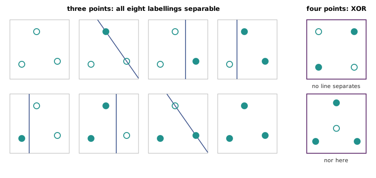
1:24:52 Vapnik’s theorem then replaces with the VC dimension : with probability at least ,
and the section’s take-away is that the number of examples needed is of the order of the VC dimension. For most classes with a reasonable parametrisation the VC dimension is roughly the number of parameters — linear classifiers in dimensions have — which is the formal version of Ng’s rule of thumb in lecture 8 that unregularised models want at least as many examples as parameters.
The VC dimension also answers the question from lecture 8 about why an SVM in an infinite-dimensional feature space does not overfit. The VC dimension of all linear separators in that space is infinite. But Ng’s answer was that the relevant class is the separators with a large margin, and for data inside a ball of radius the VC dimension of separators with margin at least is bounded in terms of , however many dimensions the feature space has. That is the sense in which minimising is regularisation.
cs229-notes4, sections 2 and 3, prove the finite-class results stated here, including the sample-complexity corollary; section 4 gives the 64-bit argument, the definition of shattering and Vapnik’s theorem. Hoeffding’s inequality is proved in the supplementary notes on Hoeffding’s inequality, via Chernoff bounds and moment generating functions.