12 Debugging ML Models and Error Analysis
Lecture 12
debugging learning algorithms, learning curves, bias versus variance, error analysis, ablative analysis
Lecture video: Lecture 12: Debugging ML Models and Error Analysis · 1:18:55
Based on the lecture by Andrew Ng — CS229, Stanford University, Autumn 2018.
A learning algorithm that does not work can be fixed in a dozen ways, and most teams pick one at random. This lecture is about picking on evidence. Each diagnostic in it makes the same move: state a hypothesis about what is wrong, then find a measurement that comes out differently depending on whether the hypothesis holds. Learning curves separate an algorithm that overfits from one that underfits. Comparing two parameter vectors on the training objective tells a failing optimiser apart from an objective that is the wrong thing to optimise. Error analysis works out which stage of a pipeline is costing the most accuracy, and ablative analysis works out which component is actually earning its keep.
Ng is explicit that this is advice for building systems that work, not for writing research papers, and that it compresses what is otherwise learned from years of projects into a handful of worked scenarios. The chapter keeps his scenarios: a spam filter, an autonomous helicopter and a face-recognition door lock.
12.1 What to try next
4:42 The running example is a spam filter. You have hand-picked a hundred words as features, trained logistic regression with a penalty on (which Ng also calls Bayesian logistic regression, since the penalty is a Gaussian prior on ; see Section 8.3), and it has 20 per cent test error. That is one mistake in every five emails, which is not good enough.
The list of things a team might try writes itself. Get more training examples. Use fewer features, since some of the hundred are probably irrelevant, or more features, since a hundred may be too few. Add features from the email header, including the routing information that records which servers the message passed through on its way to you. Run gradient descent for more iterations, or switch to Newton’s method. Change . Abandon logistic regression for an SVM or a neural network.
8:25 Ng’s observation is that teams usually pick one of these almost at random, going on what someone read the night before or what worked on the last project, and then spend days or weeks finding out whether it helped. Just writing the list down and weighing the options already puts a team ahead of most. The real fix is to work out first what kind of problem you have, because each item on the list treats only one kind. More data never hurts, but in some situations it barely helps, and finding that out by collecting it is expensive.
He also notes that he says “test error” in what follows but means error on a dev set, since decisions made by looking at the test set use it up (Section 8.4).
12.2 Learning curves
12:00 The diagnostic Ng says he uses on nearly every project is bias against variance (Section 8.1). An algorithm with high variance does much better on its training set than on the dev set. An algorithm with high bias does badly on both. The tool that tells these apart is the learning curve: training error and dev error against the number of training examples , with a horizontal line at the error you need to reach for the application to be useful. The earlier bias–variance plots had model complexity on the horizontal axis. This one holds the model fixed and varies the amount of data.
Two facts set the shape. Dev error usually falls as grows. Training error usually rises, because a small training set is easy to fit: logistic regression fits one email perfectly and five almost certainly, and a straight line passes through any two points. Only with many examples does the model start to miss some of them. Since training error is normally below dev error, the two curves approach each other from opposite sides.
Figure 12.1 draws both regimes for least-squares regression, where the expected curves have closed forms. With Gaussian features, noise variance and examples, the expected training and test mean squared errors are
Any signal the model cannot represent acts as extra noise, so in an underfitting model is replaced by the noise plus the variance it leaves unexplained. The generator checks both formulas against least squares fitted to simulated data.
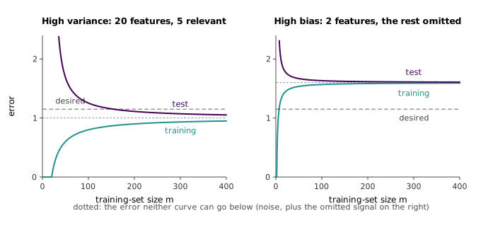
The left panel shows high variance: twenty features of which only five matter, so the fit chases noise. Ng reads two signals from a plot like this. The weaker one is that the dev error is still falling at the right edge, which suggests more data would help, but extrapolating a curve by eye is unreliable. The stronger one is the large gap between the curves. Training error sits near the target while dev error is well above it, and as the curves have to close that gap, more data will bring the dev error down. In this example it reaches the target at 155 examples.
The right panel shows high bias: two features when more are needed. Here the training error is already above the target, and since training error rises with and dev error sits above training error, no amount of data brings the dev error below the target. The curves have nearly met and both have levelled off. Collecting more data in this situation might help slightly but can never get you where you need to go.
21:12 A student asks whether these shapes depend on the data. Ng’s answer is that they assume the training, dev and test sets come from one distribution, that learning theory suggests the dev error falls roughly as , and that it need not fall to zero, because some examples are ambiguous even to an expert: a blurry X-ray, or a medical record that does not say whether the patient will survive the year.
The is worth qualifying. It is the rate in the uniform convergence bound of the learning-theory chapter, which is a worst-case guarantee across a whole hypothesis class. A particular algorithm can approach its limit faster. For least squares, Equation 12.1 puts the test error’s excess over the noise at , which falls as . Doubling the training set from 200 to 400 examples cuts the excess in the left panel from 0.112 to 0.053, a factor of 0.47, where would predict 0.71. The practical effect is that a learning curve can flatten sooner than the bound suggests, which makes Ng’s warning against extrapolating curves by eye even more apt.
12.3 Matching the fix to the diagnosis
19:08 With the diagnosis in hand, the first four items on the spam list sort themselves out. More training examples fix high variance: they are what moves the left panel’s dev curve down, and they do nothing much for the right panel. A smaller set of features also fixes high variance. Ng’s picture is a tenth-order polynomial that wiggles through every point, where dropping the high-order terms removes the wiggle. A larger set of features fixes high bias, as when a straight line is not doing well and you add a quadratic term. Header features are another way of adding information, so they are something to try against bias.
24:16 He adds advice on how to start, which the earlier chapter on Naive Bayes already raised (Section 6.4). On a new application it is very hard to know in advance what will go wrong, so implement something quick and dirty, such as plain logistic regression, run the bias–variance diagnosis on it, and let the result decide whether the next step is a bigger model or more data. The exception is a domain where you already have experience. Ng has done enough speech recognition to know roughly how much data a system needs, and someone who has read the face-recognition literature can build on it. Without that experience, the diagnosis on a simple system is the cheapest way to learn where the difficulty lies. His slides call the alternative, a careful up-front design of exactly the right features and architecture, a risk of “premature statistical optimisation”. The term parallels premature optimisation in software: effort spent on a part of the system that turns out not to be the bottleneck.
12.4 Optimisation algorithm or objective
26:30 The second diagnostic addresses the last four items on the list. Change the spam example: logistic regression now has 2 per cent error on spam and 2 per cent on non-spam. The first is tolerable, since you read the occasional spam message. The second is not, because it loses one important email in fifty. A teammate’s linear SVM gets 10 per cent error on spam but 0.01 per cent on non-spam, which is acceptable. You would still rather ship logistic regression, because it is cheaper to run and easier to update as new email arrives. What should you do?
Two quantities are in play. What you care about is a weighted accuracy on the dev set,
with a larger weight on the non-spam emails. What logistic regression maximises is something else, the regularised log-likelihood
34:09 A student asks the natural question: why not maximise directly? Because it is a sum of indicator functions. As moves, stays constant until some example crosses the decision boundary and then jumps, so its gradient is zero almost everywhere and gradient ascent has nothing to follow. The generator confirms this: at random parameter vectors, a finite-difference gradient of the weighted accuracy is exactly zero. Ng adds that maximising it exactly is NP-hard. In the learning-theory literature this is the hardness of agnostically learning halfspaces: even finding a halfspace that classifies slightly better than chance on data that some halfspace classifies almost perfectly is intractable (Guruswami and Raghavendra, 2009). So we optimise as a proxy, and the question is whether the proxy or its optimisation is letting us down.
Write for the SVM’s parameters, put in the same form as logistic regression, and for logistic regression’s. We know that . Two hypotheses could explain this. Either the optimiser has not found the maximum of , or is the wrong function to maximise. 34:40 The diagnostic is to evaluate logistic regression’s own objective at both parameter vectors and see which is higher.
Case 1: . Logistic regression was trying to maximise , yet the SVM, which was not even trying, found a point where is higher. So is not the maximiser, and the problem is the optimisation algorithm.
Case 2: . Logistic regression did better on , yet the SVM did better on . A higher value of therefore does not mean a higher weighted accuracy, so maximising is not the right thing to do. The problem is the objective.
40:09 The remaining fixes on the list now sort the same way. Running gradient descent longer and switching to Newton’s method fix the optimisation algorithm, since Newton’s method maximises the same , often much faster. Changing changes the objective, although Ng notes that in practice it is usually tuned for bias and variance instead. Switching to an SVM replaces the objective altogether. A student asks what to do once the objective is known to be wrong, and the honest answer is that nothing is automatic: you brainstorm objectives. In this example one obvious candidate is to put the weights into the log-likelihood, but the diagnostic only says which category of fix to look in.
The two cases are not symmetric, and the slides claim more for case 2 than the inequality delivers. Case 1 is a proof: is a point where is higher than where the optimiser stopped, so the optimiser has not finished. Case 2 proves that the objective is wrong, but the slides go further and read it as “BLR succeeded at maximizing ”. The inequality says only that logistic regression beat one particular point, and nothing forces that point to be anywhere near the maximum. Figure 12.2 runs the test along a training run on a toy spam problem. An SVM with errors on non-spam weighted ten times wins on weighted accuracy, 0.927 against 0.855. Logistic regression starts from , and after a single gradient step its already exceeds the SVM’s, against , so case 2 fires. Gradient ascent then needs another 31 steps to get within one per cent of the optimum at .
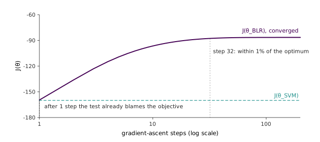
The SVM’s is low in this example partly because its parameters were never chosen to make good probabilities. Scaling leaves every prediction, and hence , unchanged but changes . Here the best rescaling only lifts from to , which is still nowhere near the optimum. So read case 2 as “the objective is wrong”, which it shows, and not as “the optimiser is fine”, which it does not. Both can be true at once. Ng’s own practice in the helicopter story below, re-running the diagnostics after each fix, covers exactly that.
12.5 The helicopter
43:17 The more complex example is the autonomous helicopter from Ng’s group, built in three steps. First build a simulator, because a simulated helicopter can crash a thousand times for free. Then choose a cost function. Ng keeps it simple for now: the squared distance between where the helicopter is and where it should be, summed over the flight. Finally run a reinforcement-learning algorithm, which the course covers in its last lectures, to find controller parameters that minimise the expected cost in the simulator.
The resulting controller flies much worse than a human pilot. Each of the three steps suggests a fix, and 48:10 each fix could absorb a PhD. Simulators can always be made more accurate: airflow around a helicopter is complicated enough that parts of it are still not fully understood, so there is almost unlimited room to improve one. The cost function may be wrong. A hovering helicopter is not level, for example: the tail rotor pushes the body sideways and the pilot tilts against it, so penalising position alone may not capture what good flight is. And the reinforcement-learning algorithm may not be finding the minimum of . Ng knows of a PhD thesis spent on helicopter simulation. That is a fine outcome if the goal is the thesis, and a poor one if the goal is a helicopter that flies.
49:50 The reasoning that cuts this down is the same as in the spam example. Suppose all three steps were sound: the simulator is accurate, the RL algorithm minimises in it, and minimising means flying well. Then would fly well on the real helicopter. It does not, so at least one of the three is false. The job is to find which, much as one isolates a bug in a large program by bisecting it instead of reading the whole code base. Figure 12.3 lays out the two tests.
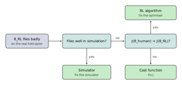
51:48 First, fly in the simulator. If it flies well there and badly in reality, the RL algorithm did its job on the problem it was given, and the simulator is what differs from the real world. A student asks whether the reverse can happen, flying badly in simulation and well in reality. Ng says it is rare, and when it happens he still works on the simulator. His group deliberately adds noise to its simulators so that a controller robust to the simulated noise is more likely to be robust to real disturbances, and a controller that does well in reality but not in simulation can mean that too much noise was added.
54:40 If the controller also flies badly in simulation, compare it with the human on the RL algorithm’s own cost: record the human pilot’s flight and evaluate the same squared error. If , the human achieved a lower cost than the algorithm found, so the algorithm is not minimising , and that is the part to improve. If , the algorithm reached a cost at least as low as the human’s while flying worse, so a low does not mean good flight, and the cost function is wrong. The same asymmetry as in the previous section applies here, now with the human as the witness point.
58:10 In the actual project, Ng says, the bottleneck moved around. For a few weeks the diagnostics pointed at the simulator; once it was good enough they pointed at the RL algorithm, and later at the cost function. Running them again after each round of work is what kept the team on the part that mattered. The cost function turned out to be the hard one, because it is not obvious how to write down mathematically what a good banked turn is. His student Adam Coates found a way through learning the target trajectory from several imperfect expert demonstrations, work published as Learning for Control from Multiple Demonstrations (Coates, Abbeel and Ng), which was presented in the award-paper session of ICML 2008.
12.6 Error analysis
1:01:24 Many applications are not one learning algorithm but a pipeline of them. Ng’s example is a camera by a door that unlocks for authorised people. The image goes through background removal, which with a fixed camera can be as simple as keeping the pixels that changed. Then a face detector finds the face, separate components segment the eyes, nose and mouth (the eyes being a particularly strong cue for identity), and logistic regression on those features decides whether to open the door. Ng adds that pipelines like this are what small data sets call for. His teams often get good results from a hundred examples, but only through more careful design than a single end-to-end model needs.
When such a system reaches 85 per cent accuracy, which component should you work on? 1:06:04 Ng tells the story of someone who chose background removal, which can be made almost arbitrarily sophisticated by modelling the trees and bushes moving behind the subject, and wrote a whole PhD thesis on it, without improving the face recognition he set out to build.
1:07:50 Error analysis answers the question by substituting ground truth. On the dev set, replace the output of background removal with a perfect one, labelled by hand, and measure the system’s accuracy. Then also give it perfect face locations, then perfect eye, nose and mouth segmentations, and finally perfect labels, which must give 100 per cent. Figure 12.4 shows the lecture’s numbers.
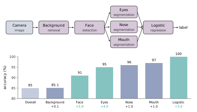
Perfect background removal is worth 0.1 points, so a thesis on it can change the door lock’s accuracy by at most that much. Perfect face detection is worth almost six points and perfect eye segmentation another four, so those are the components to work on, in parallel if the team is big enough. The fifteen points between 85 and 100 per cent are divided among the stages, and each stage’s share bounds what improving it could gain.
Two student questions sharpen this. 1:11:13 Should the substitution be cumulative, as in the figure, or one component at a time? Ng’s answer is that either will do, that they usually agree, and that if you suspect they will not, you should run both. Ablation, below, gives a concrete case where they do not. 1:13:21 What if giving a component perfect output makes the system worse? That should be rare, and Ng’s advice is not to gloss over it. Treat it like a button that misbehaves only when the mouse hovers over it: an anomaly to understand, not one to dismiss because users will not notice. He also notes that the numbers are a guide to prioritisation, to be combined with a judgement of how hard each component would be to improve. They do not settle the decision by formula.
12.7 Ablative analysis
1:14:35 Error analysis explains the gap between where a system is and perfection. Ablative analysis explains the gap between where it is and a much worse baseline. Back to spam: suppose a good classifier has been built by adding clever components to plain logistic regression. These are spelling correction (spammers misspell words to get them past the tokeniser), features of the sending host, email header features, a parser for the email text, a JavaScript parser and features from images. Plain logistic regression gets 94 per cent and the full system 99.9. What accounts for the difference?
Remove components one at a time, cumulatively, and record the accuracy after each removal:
| Removed | Accuracy | Drop |
|---|---|---|
| nothing (full system) | 99.9 % | |
| spelling correction | 99.0 % | 0.9 |
| sender host features | 98.9 % | 0.1 |
| email header features | 98.9 % | 0.0 |
| email text parser features | 95.0 % | 3.9 |
| JavaScript parser | 94.5 % | 0.5 |
| features from images | 94.0 % | 0.5 |
The text-parser features account for most of the gain. For a paper or a project report this is the result to state: the report then explains why the system works, not just that it does. If you are going to work on spam for years, it tells you where to invest. 1:18:21 The last question of the lecture asks how to choose the order of removal. There is no systematic way, Ng says, so if in doubt use the non-cumulative version: remove one component, put it back, remove the next.
1:17:03 He says that the two versions usually give similar insight. Usually they do, but there is a common case where they cannot, and Table 12.1 hints at it. Removing the header features costs nothing after the sender-host features are gone, which is what happens when two components carry largely the same information. The generator builds this case exactly. Two classes are Gaussian with a shared covariance, and there are four features: “sender host” and “email header” are separate measurements of the same signal (correlation 0.95), “text parser” is a strong independent feature and “JavaScript” a weak one. For this model the best classifier on any subset of features has accuracy , where is the Mahalanobis distance between the class means on that subset, so every ablation can be computed in closed form.
| Feature | Leave one out | Cumulative, sender host first | Cumulative, header first | Averaged over orders |
|---|---|---|---|---|
| sender host | 0.001 | 0.001 | 0.055 | 0.070 |
| email header | 0.001 | 0.055 | 0.001 | 0.070 |
| text parser | 0.087 | 0.172 | 0.172 | 0.130 |
| JavaScript | 0.004 | 0.060 | 0.060 | 0.019 |
Leave-one-out says the sender-host and header features are each worth a tenth of a point, since either one can stand in for the other. Yet removing both together costs 5.6 points. Cumulative removal hands the whole 5.5 to whichever of the two is removed second, so the conclusion depends on an order that was chosen arbitrarily. The final column, the drop averaged over every removal order (the Shapley value from cooperative game theory), splits the credit evenly. Its entries add up to the full 28.8 points, as any single removal order’s do. Leave-one-out’s add up to only 9.4, because the credit the two redundant features share is counted for neither.
Order also matters for weak features: JavaScript looks worthless with everything else present and worth six points once the stronger features are gone. None of this makes ablation less useful. It means that when two components could plausibly duplicate each other, you should remove them together as well as separately before concluding either is dead weight. Error analysis has the same problem in reverse when stages interact: giving one stage perfect input may help little until another stage is fixed too.
This lecture has no class notes. Its slides are Ng’s Advice for applying machine learning, and the course’s error-analysis section handout covers the same pipeline example.