4 Perceptron and Generalized Linear Models
Lecture 4
perceptron, exponential family, generalized linear models, softmax regression, cross-entropy
Lecture video: Lecture 4: Perceptron and Generalized Linear Model · 1:22:02
Based on the lecture by Anand Avati — CS229, Stanford University, Autumn 2018.
Lectures 2 and 3 derived linear regression and logistic regression separately, and both ended with the same update, . This lecture, given by Anand Avati while Ng was away, explains why. Both models are instances of a generalized linear model: pick a distribution for from the exponential family, let its natural parameter be a linear function of , and the hypothesis, the likelihood and the update all follow — the same update every time, with only changing. The sigmoid, which lecture 3 introduced without justification, falls out of this recipe once is assumed Bernoulli. The lecture opens with the perceptron, which has the same update for a different reason, and closes with softmax regression, which extends logistic regression to many classes.
4.1 The perceptron
1:35 The perceptron replaces logistic regression’s sigmoid with a hard threshold, if and otherwise, so outputs a label rather than a probability. The update is the one from lecture 3, written for one example at a time:
Avati reads it from the inside out. Since and are both 0 or 1, the bracket can take only three values: 0 when the prediction is right, so nothing happens; when a positive example was called negative; and in the opposite case. A correctly classified example therefore leaves alone, and a misclassified one adds or subtracts a multiple of itself.
7:27 The geometric picture makes that rule look inevitable rather than arbitrary. The decision boundary is the line perpendicular to , and is positive for inputs on the side points toward. We want to have a positive dot product with the positive examples and a negative one with the negative examples — to be similar to the first and dissimilar to the second. When a positive lands on the wrong side, the most naive way to make more like is to add a bit of to it. That rotates toward , and the boundary rotates with it (Figure 4.1).
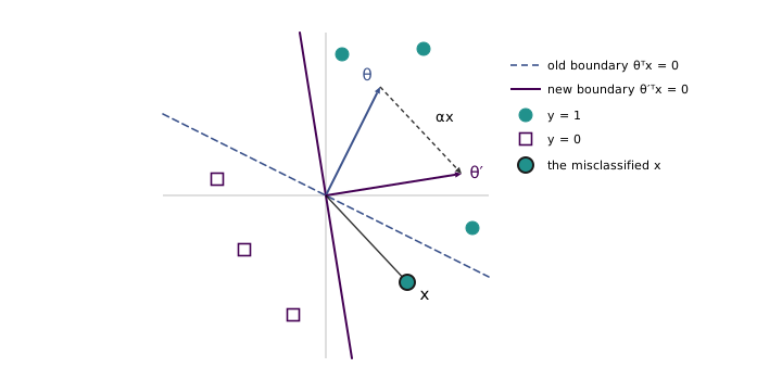
figures/04-perceptron-glm/make_diagrams.py.
The lecture calls “some small learning rate”, but for the perceptron as usually run it has no effect at all. Starting from , every update adds , so is always times a sum of examples, and the sign of — the only thing the prediction depends on — does not depend on . The generator checks this: on a separable set of 40 points, and make the same 8 mistakes in the same order and finish with parameter vectors that differ by exactly the factor of 1000. The learning rate starts to matter only if it changes over time, which is where a student question led.
12:39 Asked why the perceptron is not used in practice, Avati gives two reasons. It has no probabilistic interpretation: it draws a boundary but says nothing about how confident it is. And it has a famous limitation. The perceptron was celebrated in the late 1950s as a model of the brain (Rosenblatt, 1958); the 1969 book Perceptrons by Marvin Minsky and Seymour Papert (the lecture remembers it as a paper by Minsky) set out what a single linear threshold unit cannot compute, and the smallest example is XOR — two positive and two negative points at the corners of a square, diagonally opposite, which no line separates. Interest in the model collapsed afterwards.
13:39 A second question asked when to stop training. If the data are linearly separable, the answer is a theorem the lecture does not state: the perceptron stops making mistakes after finitely many updates. If every and some unit vector separates the classes with margin , the number of mistakes is at most , whatever the order of the examples (Novikoff, 1962). On the generator’s 40 points the bound is 55 and the perceptron makes 8. If the data are not separable, it never settles — on XOR it is still making mistakes on all four points in the thousandth pass — so Avati’s practical advice is to anneal: shrink with every example until stops moving much. That is exactly the case where is no longer irrelevant, since later updates then count for less than earlier ones.
13:31 Avati also offers the cleanest way to place the perceptron beside the previous lecture: logistic regression is a soft version of it. The step function is the limit of as the slope grows (Figure 4.2); at the two already differ by less than 0.003 everywhere outside . What the sigmoid buys in exchange for that softness is a likelihood, and with it everything that follows.
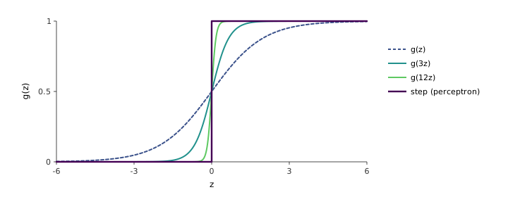
figures/04-perceptron-glm/make_diagrams.py.
The perceptron is the short digression of cs229-notes1, section 6, which presents it only as an algorithm; the mistake bound above is not in the 2018 notes.
4.2 The exponential family
14:53 The exponential family is a class of distributions with convenient mathematics, and it is the bridge to generalized linear models. A distribution belongs to it if its density (or, for discrete , its probability mass function) can be written
Avati names each piece. The variable is called , not , on purpose: these distributions will model the output of a supervised problem, and enters only when the model is built. is the natural parameter. is the sufficient statistic, in the statistician’s sense, but for every distribution in this course , and the lecture tells the reader to make that substitution and move on. is the base measure, which may depend only on ; and is the log-partition function, which may depend only on . In most of the course and are scalars; softmax will need a vector .
18:48 The name of explains its job. Moving it out of the exponent gives , so is the normalising constant — the partition function — that makes the density integrate to one, and is its log. That has a consequence worth making explicit, because the lecture says one can choose , and freely as long as the result integrates to one. The condition is not a side constraint on ; it determines it. Once and are fixed,
with a sum in place of the integral for discrete . Choosing and chooses the family; comes with it. The generator confirms, for the three families below, that the read off by pattern matching equals this normaliser computed by brute-force summation.
21:44 To show that a familiar distribution is a member, write its density in the usual form and massage it until it matches Equation 4.2. For the Bernoulli with mean , the density — an “if–else written in maths”, as Avati puts it, since it equals when and when — becomes, after wrapping it in ,
Matching term by term gives , , the natural parameter , and . 26:14 Inverting the expression for gives
the sigmoid, which arrives here without being asked for. Substituting it into gives , now a function of alone as the definition requires.
28:41 The Gaussian works the same way once its variance is fixed. With — and lecture 3 showed that the variance has no effect on the fitted in least squares, so nothing is lost —
so and . A student asked what happens if the variance is unknown: the Gaussian is still in the family, but becomes a two-dimensional vector and . The Poisson, which the lecture uses later without deriving, fits the same mould: has , and .
The Bernoulli and Gaussian derivations are cs229-notes1, section 8, which also lists the multinomial, Poisson, gamma, exponential, beta and Dirichlet as members.
4.3 Why the exponential family is convenient
33:10 Three properties make the family worth the trouble, and Avati states them without proof — they are an exercise in the first problem set. First, maximum likelihood in the natural parameter is a concave problem, so it has no spurious local maxima; the negative log-likelihood, its cost-function form, is convex. Second and third, the log-partition function produces the moments by differentiation:
35:08 The point Avati makes about these is practical: computing a mean or a variance normally means integrating against the density, and here it means differentiating a single function, which is far easier. For the Bernoulli, and ; for the Gaussian, and ; for the Poisson, both derivatives are , the textbook fact that a Poisson’s mean equals its variance. The generator checks all three by computing and by finite differences and the mean and variance by summing over the support. The first property follows from the third: a variance is never negative, so is convex, and the log-likelihood is linear minus convex, which is concave. 36:06 When is a vector, as for a Gaussian with unknown variance, a student asked how this generalises; the gradient of gives the mean of and its Hessian the covariance.
4.4 Generalized linear models
36:35 A generalized linear model attaches the inputs to an exponential-family distribution, and the lecture frames it as three design choices.
- is distributed according to some member of the exponential family, with natural parameter .
- The natural parameter is linear in the input: , with .
- At test time, the prediction for is the mean of that distribution: .
38:36 The first choice is the modelling decision, and it is dictated by what kind of quantity is. Real-valued outputs such as house prices call for a Gaussian; binary labels for a Bernoulli; counts — non-negative integers, such as the number of visitors to a website — for a Poisson; positive reals such as a volume or the time until an event for a gamma or an exponential. Avati warns that the exponential distribution and the exponential family are different things, though the first is a member of the second, and the list ends with distributions over probabilities, the beta and the Dirichlet, which mostly appear in Bayesian statistics. Whether a GLM is a classifier or a regressor is therefore not a property of GLMs at all: it is decided by the distribution put in the first slot.
42:55 The picture to keep in mind has two halves. On the left is a linear model: goes in, a learnable multiplies it, and out comes a number. On the right is a distribution from the exponential family, and that number becomes its natural parameter. 45:40 Only is learned. A student asked whether training adjusts the distribution’s parameters, and the answer separates two uses of the word “parameter”: is not a variable that gradient descent touches, it is the output of the linear model for one particular . Training is maximum likelihood over ,
which is concave in because it is concave in and is linear in .
48:46 Here the recipe pays off. One would expect each new distribution to need its own algebra: write as a function of , differentiate, simplify. It does not, because for every GLM built this way the stochastic gradient-ascent update is
with the only thing that changes. The derivation is one line: the log-likelihood of one example is , and its gradient is , which by Equation 4.4 is . This is why linear regression, logistic regression and Poisson regression share an update: the first is the Gaussian GLM with , the second the Bernoulli with , the third the Poisson with . The generator checks the expression against a numerical gradient of the log-likelihood for all three.
“Every GLM” carries a qualification the lecture leaves implicit: the identity holds because the natural parameter itself is set to . A model that instead connects to the mean through some other function does not inherit it. The probit model of lecture 3, with the standard normal CDF, is a Bernoulli model with exactly the same shape, and the update that looks right for it — Equation 4.5 with — is not its gradient: at a test point on synthetic data it has the right direction but a length off by 41 percent. That would be harmless if it only rescaled the step, but it also moves the place where the step vanishes. Iterated to convergence, the look-alike update stops at , while the probit maximum-likelihood estimate is . The two links are close, so the error is small, but the algorithm is now solving a different equation from the one it claims to.
50:43 For batch training, sum the update over the examples. Asked about Newton’s method, Avati calls it probably the most common way to fit a GLM, provided the number of features is below a few thousand, so that the Hessian is affordable — the same rule of thumb Ng gave in lecture 3. Concavity is what makes it safe: on a Poisson regression with 200 synthetic counts, Newton’s method reaches the maximum in 7 iterations, at the same that plain gradient ascent eventually finds.
4.5 Three parametrisations
52:03 The lecture pauses on terminology, because a GLM has three sets of numbers called parameters and they are easy to confuse (Figure 4.3). The model parameters are what learning adjusts. The natural parameter is the linear model’s output, one per example. The canonical parameters are the ones the distribution is usually written in: for a Bernoulli, (and ) for a Gaussian, for a Poisson. The step from to is linear by design choice 2. The step from to the mean has a name: is the canonical response function, and its inverse is the canonical link function.
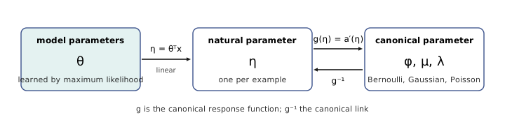
56:23 With the vocabulary in place, logistic regression stops being a choice and becomes a consequence. For a binary label the natural distribution is the Bernoulli; design choice 3 says the hypothesis is its mean, ; and Equation 4.3 says with . Lecture 3 pulled the logistic function “out of thin air” because it squashes the real line into . Here, as Avati puts it, it simply pops out: the sigmoid is the canonical response function of the Bernoulli. The same steps applied to the Gaussian return , ordinary least squares.
The idea and the name are due to Nelder and Wedderburn (1972), who showed that one fitting procedure covered regression models that had been treated separately.
cs229-notes1, section 9, constructs the GLM from the same three assumptions and derives ordinary least squares (9.1) and logistic regression (9.2) from them.
4.6 What the assumptions say about the data
1:00:03 Avati’s last pass over GLMs draws the assumptions as a story about how the data were generated. For the Gaussian, take a line ; at every , stand a unit-variance Gaussian on the line; and draw each training from the Gaussian above its (Figure 4.4, left). Learning runs the story backwards: each choice of is a different line, and maximum likelihood picks the line from whose Gaussians the observed points were most likely to have come.
1:04:50 For classification the story has one more step. The line now gives , which can be any real number; passing it through the sigmoid gives , the probability that at that ; and each label is a coin flip with that bias, so labels are mostly 0 where the curve is low and mostly 1 where it is high (Figure 4.4, right). Logistic regression asks which would have produced a sigmoid from which these labels were most likely drawn.
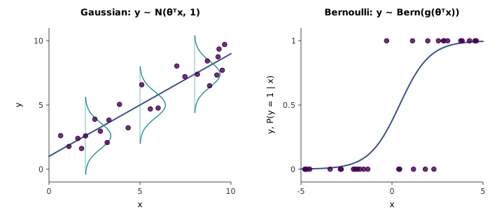
figures/04-perceptron-glm/make_diagrams.py.
4.7 Softmax regression
1:07:58 Softmax regression extends logistic regression to classes. The notes present it as one more GLM, built on the multinomial distribution; the lecture deliberately takes another route and presents it as cross-entropy minimisation, an interpretation worth having because it is how classifiers with thousands of classes are usually described.
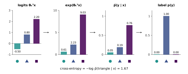
1:11:04 The labels are one-hot vectors: a vector of zeros with a single 1 in the position of the correct class. Where logistic regression had one parameter vector, softmax has one per class, , which together form an matrix. For an input , each class gets a score , called a logit, which can be any real number. 1:16:24 To turn the scores into a probability distribution over classes, exponentiate them, which makes them all positive, and divide by their sum, which makes them add to one:
1:19:09 The label is read as a distribution too, , which puts probability 1 on the correct class. Learning makes look like by minimising the cross entropy between them,
where the sum collapses because is zero everywhere except at the true class . (The minus sign is missing from the board the first time; it belongs there, since the loss has to be non-negative.) Figure 4.5 follows one example through the pipeline: an input whose true class is triangle but which scores highest for square receives and a loss of 1.67. The last expression in Equation 4.7 is the negative log-likelihood of a multinomial model, so the lecture’s route and the notes’ arrive at the same objective. Its gradient for class is , the same “prediction minus truth, times input” shape as Equation 4.5; and with the softmax probability of class 1 is exactly , logistic regression with .
figures/04-perceptron-glm/make_diagrams.py.
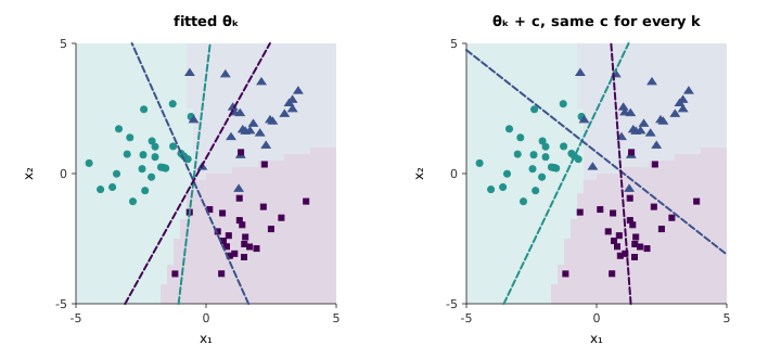
1:12:53 That two-class reduction exposes something the board picture hides. The lecture draws one line per class, , with each class’s own region on the positive side, as though each carves out its class independently. But Equation 4.6 is unchanged if the same vector is added to every : the factor cancels between numerator and denominator. Only the differences matter, so the decision boundary between two classes is , and the individual lines can be moved anywhere without changing a single prediction (Figure 4.6). On the fitted model in the figure, the board’s picture — exactly one positive score, and it belongs to the predicted class — holds on only 45 percent of the plotted square even before any shift. This redundancy is why the official notes give softmax only parameter vectors and fix : the -th vector adds nothing a shift could not remove.
figures/04-perceptron-glm/make_diagrams.py.
cs229-notes1, section 9.3, derives softmax regression as the GLM for the multinomial distribution, with a -dimensional indicator vector, and arrives at the same hypothesis and log-likelihood.