2 Linear Regression and Gradient Descent
Lecture 2
linear regression, gradient descent, stochastic gradient descent, least squares, normal equations, LMS update
Lecture video: Lecture 2: Linear Regression and Gradient Descent · 1:18:17
Based on the lecture by Andrew Ng — CS229, Stanford University, Autumn 2018.
The second lecture builds the first complete learning algorithm of the course and then solves the same problem a second way. Linear regression predicts a number as a weighted sum of features; the weights are chosen to make the squared error on the training set as small as possible; and that minimum can be found either by walking downhill on the error surface, one gradient step at a time, or by solving a linear system for it directly. Gradient descent is the half that matters later: the normal equations work for linear regression and its weighted variant and nothing else in the course, while the walk downhill reappears in logistic regression, generalised linear models and neural networks. Ng uses this lecture to set up the vocabulary all of them share — hypothesis, parameters, cost function, learning rate — and it is worth getting that vocabulary straight here, where the mathematics is still simple enough to check by hand.
2.1 The housing problem and the hypothesis
1:55 The running example is the one that closed lecture 1: predict the asking price of a house from its size. Ng’s data are real, a few dozen listings from Portland, Oregon collected off Craigslist — a 2,104 ft² house listed at $400,000, a 1,416 ft² one at $232,000, and so on — and the task is to fit a straight line through them.
Before writing any formula he describes the shape every supervised algorithm in the course will have. A training set goes into a learning algorithm, and what comes out is a function, by convention called the hypothesis , which takes the size of a house it has never seen and returns an estimated price. The learning algorithm’s job is to produce ; ’s job is to make predictions. 4:43 The first design decision is therefore not how to fit, but how to represent , and for linear regression the answer is
with the size and the number of bedrooms. Ng concedes the point a mathematician in the room would raise: with the term this is an affine function, not a linear one, and machine learning calls it linear anyway.
The intercept is awkward to carry around, so it is absorbed into the sum by inventing a feature that is always one, . Then and are both vectors in , and
The rest of the notation is fixed here for the whole quarter. The are the parameters, and choosing them is all that learning means for this model. is the number of training examples (rows of the table), the number of features (two here, so and are three-dimensional), the input features and the output or target. The -th training example is written , and the superscript in parentheses is an index into the table, not a power: is the size of the first house. Ng is open that some of this terminology is an accident of history — he does not think “hypothesis” is a good name, but someone used it in a paper decades ago and the field is stuck with it.
2.2 The least-squares cost
14:41 “Choose so that is close to on the training examples” needs a number that measures closeness, and Ng builds it one piece at a time on the board: the squared difference between prediction and truth for one house, summed over all houses, with a factor of one half in front:
is the cost function, and linear regression — ordinary least squares — is the choice of that minimises it. The one half changes nothing about where the minimum is; it is there so that the 2 brought down by differentiating a square cancels it, as it will in Section 2.4.
16:39 The question Ng says he is asked most often is why the error is squared rather than taken in absolute value or raised to the fourth power. His answer here is a deferral with a hint: squared error corresponds to assuming the noise in is Gaussian, and linear regression turns out to be one member of a family, the generalised linear models, in which that choice is derived rather than assumed. The next lecture makes the Gaussian argument precise.
2.3 Gradient descent
18:27 The algorithm for minimising starts from some initial — the zero vector is a reasonable default, a random start is also fine — and keeps changing in a way that lowers .
19:40 Ng’s picture for it is a landscape. Put and on the two horizontal axes and as the height (with three parameters the surface lives in four dimensions, which is why the picture uses two). Stand at the starting point, turn through 360 degrees, and ask: if I took one tiny step, which direction would take me downhill fastest? Take that step, look around again from the new spot, and repeat.
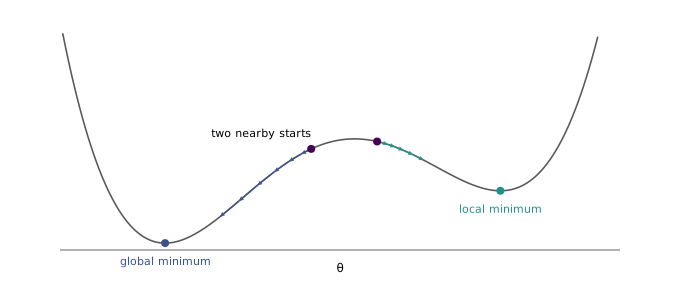
22:03 The picture also exposes the method’s weakness. On a landscape with more than one valley, where you end up depends on where you start: begin a few steps to one side and the same procedure walks you into a different local minimum (Figure 2.1). For linear regression this turns out not to matter, for a reason Section 2.5 gives, but it matters a great deal for most of what comes later in the course.
figures/02-linear-regression/make_diagrams.py.
23:54 Formally, one step of gradient descent updates every parameter at once:
The partial derivative gives the direction of steepest ascent, so subtracting a multiple of it goes downhill. The multiple is the learning rate, which sets the size of the step. The := is assignment, and Ng is deliberate about it: increments , whereas asserts a fact, and he promises never to write . Throughout the update, the training set is fixed and is a fixed function of ; only moves.
26:04 A student asked at once how to choose . “There’s a theory and there’s a practice,” and the practice, to laughter, is . The serious version followed: if the features are scaled to roughly , start at and try larger and smaller values to see which drives down fastest. Section 2.5 says why the scaling clause is not optional.
2.4 The LMS update
27:27 To run Equation 2.4 the partial derivative has to be computed, and Ng does it for a training set of a single example first, so that the sum does not get in the way. The chain rule brings the 2 down from the square, where it cancels the half, and leaves the derivative of what was inside:
Of all the terms in the expanded sum only depends on , so every other term differentiates to zero and this one to .
31:43 With examples, the derivative of a sum is the sum of the derivatives, and the full algorithm is
This is the least-mean-squares or Widrow–Hoff rule, and it reads well once written out. Each example pushes in proportion to its own error: a house whose price is already predicted almost exactly barely moves the parameters, one that is badly mispredicted moves them a lot, and the push on is weighted by how large the feature was for that house. The generator behind this chapter checks Equation 2.6’s sum against finite differences of on the housing data, and it agrees.
The same derivation, and the remark that the update is proportional to the error, are in cs229-notes1, section 1.
2.5 A bowl, and the learning rate
33:52 The local-minimum worry of Figure 2.1 disappears for this cost. is a sum of squares of functions linear in , so it is a quadratic in , and a quadratic of this kind is a single bowl: its only local minimum is the global one. Looked at from above, its contours are nested ellipses, and Ng adds a fact he half-remembers from school — “I think it’s true” — that each step of steepest descent crosses the contour it starts on at right angles. It is true: the gradient is normal to the level set through any point, and the generator confirms it on the housing cost to within a cosine of 0.003.
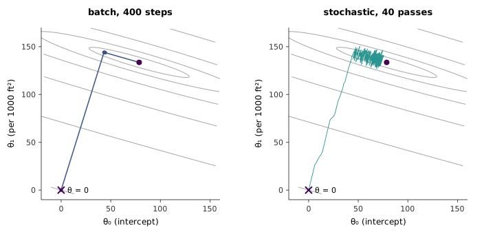
What the board picture does not show is how thin the bowl can be. Figure 2.2 runs gradient descent on synthetic housing data shaped like Ng’s, with size in thousands of square feet, starting from . The first step drops almost straight across the contours into the floor of a long valley; every step after that inches along the floor towards the minimum, and it takes more than four hundred of them to bring the intercept within $500 of its final value. The ratio of the bowl’s steepest to its shallowest curvature — the eigenvalues of , in the notation of Section 2.8 — is about a hundred here, and gradient descent’s pace is set by the shallow direction while its step size is capped by the steep one.
figures/02-linear-regression/make_diagrams.py.
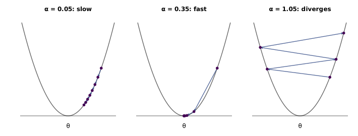
That cap is the precise version of Ng’s 36:08 advice on the learning rate. Too small and the algorithm needs very many iterations; too large and each step overshoots the minimum, lands higher on the far side, and diverges (Figure 2.3). For a quadratic the boundary is exact: with the largest eigenvalue of , gradient descent converges for and diverges above it, which the generator checks on both sides of the line. His practical rules follow from watching rather than computing eigenvalues. If goes up over iterations, the learning rate is almost certainly too large. And rather than search finely, try values on a roughly doubling scale — 0.01, 0.02, 0.04, 0.08 — and keep whichever drives down fastest.
figures/02-linear-regression/make_diagrams.py.
The same bound explains the feature-scaling clause in “set it to 0.01”. On the synthetic data with size measured in raw square feet, is so large that the stable range ends at , and diverges immediately; with size rescaled to about the limit is about , and is comfortably safe. One further caveat follows from writing as a sum. grows with , so the safe learning rate shrinks as the training set grows, and that works on 47 houses will not on 47,000. Many implementations average the squared error instead of summing it, which removes that dependence; the minimum is unchanged either way.
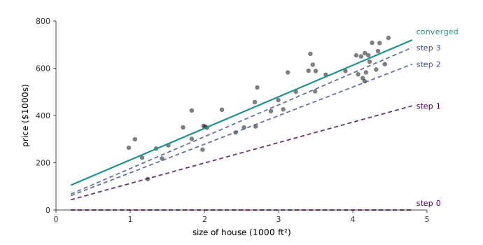
37:14 Ng’s second view of the same run is in the data rather than in parameter space. With the hypothesis is the horizontal line , predicting every house free; each step of gradient descent replaces it with a line that fits a little better, until it settles on the least-squares fit (Figure 2.4).
figures/02-linear-regression/make_diagrams.py.
39:30 A student asked why the update subtracts times the gradient rather than adding it. Ng’s suggestion was to work one case by hand, and it settles the matter: take at . The derivative there is (Ng said 1 at the board; the sign is what matters), positive, and to reach the minimum at zero has to decrease — so the step must go against the gradient. Adding it would climb.
2.6 Stochastic gradient descent
41:05 Equation 2.6 is called batch gradient descent because every single update looks at the whole training set as one batch. That is its weakness. If is the size of the US census rather than of a Craigslist scrape — Ng mentions training on hundreds of millions of examples — then one step requires a full pass over the data, possibly terabytes read from disk, before moves at all, and convergence can take hundreds or thousands of such steps.
44:13 Stochastic gradient descent updates after every example instead:
46:02 In Ng’s words it looks at one house and adjusts the parameters to predict that house better, then the next house, then the next. No single house’s gradient points straight at the minimum, so the path is noisy, but on average it heads downhill, and it starts making progress after the first example rather than after the millionth. The price is that it never quite converges: because each update chases a different house, keeps wandering around the minimum, as on the right of Figure 2.2. For a large dataset that trade is almost always worth making.
The questions from the room fill in how it is used in practice. Asked 47:58 whether one could start stochastic and switch to batch near the end, Ng said yes, and that it does no harm — but that people rarely bother, because batch steps on a large dataset are too slow to be worth it, and because the parameters stochastic gradient descent ends near are usually perfectly good even if they are not exactly the global minimum. The middle ground, which he names and leaves to CS230, is mini-batch gradient descent, which updates on a hundred or so examples at a time. What is common instead is 50:03 to decrease the learning rate slowly over time: the oscillations shrink with the step size, so ends up bouncing around a smaller region closer to the minimum. Asked when to stop, his answer was to plot over time and stop when it stops going down — easy here, where there are no local optima to confuse the picture, and much harder for the neural networks later in the course.
51:35 The last question was whether stochastic gradient descent’s learning rate should be times batch’s. No, Ng said, it is usually much bigger, since otherwise it would be as slow as batch. The arithmetic behind that answer is worth having. Because is a sum, a full pass of Equation 2.7 at rate adds up, to first order in , to one batch step at the same ; the generator confirms the gap between them shrinking as does. Dividing by would therefore make a whole pass of stochastic updates worth only of a batch step. And a single-example update tolerates a far larger rate in the first place: its stability limit is rather than of the whole of , which on the synthetic housing data is a factor of about 25 more room.
51:51 Ng’s own rule of thumb closes the topic. With a dataset of hundreds or thousands of examples, where a pass is cheap, he would almost always use batch gradient descent, because it is one less thing to fiddle with — no oscillating parameters to worry about. When the data are too large for that, almost everyone uses stochastic gradient descent or something like it.
2.7 Matrix derivatives and the trace
53:25 For linear regression, and for exactly linear regression — none of the models of the following lectures beyond its weighted variant in lecture 3 — there is a way to skip the iterations altogether and jump to the minimum in one step. Deriving it means setting the gradient of to zero and solving, and Ng’s aim is to do that “in roughly four lines of linear algebra rather than pages and pages”, which takes a little notation first. In his experience, he says, the right notation is what makes such problems tractable.
56:02 For a function , the derivative with respect to the vector is the vector of partial derivatives,
and more generally, for a function that maps an matrix to a real number, is the matrix whose entry is . Ng’s example 58:32 is a made-up function of a matrix, , so that applied to the matrix with rows and is , and
A student asked whether the vector definition was a special case of the matrix one; it is — a vector is an matrix, and the two agree.
1:03:35 The second tool is the trace of a square matrix, the sum of its diagonal entries, . Transposing a matrix leaves its diagonal where it was, so . The trace of a product is unchanged by moving the last factor to the front, and , and its derivative has a clean form:
1:06:23 Ng then gives one identity as the matrix analogue of , a rule to be used without re-deriving it every time, the way one uses the derivative of . The analogy is a good way to remember the shape of the result, but the generator caught that the shorthand needs a condition the board left out:
which equals only when is symmetric. For a random non-symmetric , the numerical gradient matches Equation 2.11 and misses by a visible margin; for the symmetric part of the same the two coincide. In the derivation that follows is and the matrix playing the role of is , which is symmetric, so nothing goes wrong, but the general rule is the one with . The official notes state the fully general version, , which reduces to Equation 2.11 when is the identity.
2.8 The normal equations
1:08:39 To write with matrices, stack the training inputs as the rows of the design matrix , an matrix whose -th row is , and stack the targets into a vector . Then is the vector of every prediction at once, since its -th entry is , and is the vector of every error. A vector dotted with itself is the sum of its squared entries, , so
1:13:08 Now take the gradient and set it to zero. Expanding the product the way one expands gives four terms, . The last does not depend on ; the middle two are the same scalar, each the transpose of the other; and the trace rules of Section 2.7 differentiate the first to and the middle pair to . Halving,
This is Equation 2.6’s sum written in matrix form, which is a useful check on both. 1:16:19 Setting it to zero gives the normal equations,
A few matrix products land on the global minimum of the bowl in one step, the same point that gradient descent spends hundreds of steps approaching in Figure 2.2; the generator runs both and confirms they agree to six decimal places. On the real Portland data the official notes report the fit , : about $71,000 plus $134.50 per square foot.
1:17:01 The common question is what to do if is not invertible. That usually means the features are linearly dependent — redundant — and the matrix pseudo-inverse will still return a sensible answer. But Ng’s preferred fix is diagnostic: a singular most often means the same feature is in the data twice (size in square feet and size in square metres, say), and the right move is to find the duplicate and drop it. With a feature duplicated, every way of splitting its weight between the two copies gives exactly the same predictions and the same , which is why no single can be picked out by the equations; the generator checks this on a copy of the housing data with the size column repeated.
His last answer, to a final question on how to choose the learning rate, came back to where Section 2.3 left it: it is empirical, and most people try several values and keep the one that works.
The matrix-derivative identities and the full derivation of the normal equations, including the trace manipulation Ng skips, are in cs229-notes1, sections 2.1 and 2.2. Section 3 justifies the least-squares cost as maximum likelihood under Gaussian noise, which is where the next lecture begins.