6 Support Vector Machines
Lecture 6
Laplace smoothing, multinomial event model, support vector machines, functional margin, geometric margin, optimal margin classifier
Lecture video: Lecture 6: Support Vector Machines · 1:20:57
Based on the lecture by Andrew Ng — CS229, Stanford University, Autumn 2018.
Naive Bayes, as lecture 5 left it, breaks the first time a word turns up that the training set never contained: every class gets probability zero and the posterior is . The fix is to add one to every count, and that rule, Laplace smoothing, is what a Bayesian with a uniform prior would compute anyway. With smoothing in place the lecture builds a second naive Bayes for text, the multinomial event model, which counts how often each word occurs instead of only whether it does, and then steps back to argue that an algorithm this cheap is the right first thing to build. The second half starts the support vector machine. Before kernels, an SVM is a linear classifier chosen for one property: of all the lines that separate the training data, it takes the one that stays furthest from every example. Most of the work is in defining “furthest” so that it cannot be gamed.
6.1 Laplace smoothing
4:42 Ng’s example of the zero problem is a word that is new to your inbox but not to the world. Suppose “NIPS”, the machine learning conference, is word 6017 of a 10,000-word vocabulary, and nobody has yet e-mailed you about it. The maximum likelihood estimates from lecture 5 are fractions of e-mails containing the word, so both and come out as . 8:03 Months later your project team writes about submitting to NIPS. The product now contains a factor of zero for both classes, and the classifier’s posterior is . The division by zero is the visible symptom; the underlying error, Ng says, is statistical — estimating the probability of something as zero because you have not seen it yet.
9:58 He sets spam aside to make the point with a smaller example. One season, Stanford’s football team played four out-of-state games — Wake Forest, Oregon State, Arizona and, Ng adds for the room, Caltech — and lost all four. You followed them to every one. What is the chance they win the next? Maximum likelihood counts wins over games played, : absolute certainty of a loss, which is unkind and also unreasonable. 11:59 Laplace smoothing pretends you saw one more of each outcome than you did — one extra win and one extra loss — so the estimate becomes .
12:58 The rule is not arbitrary. Laplace derived it for the probability that the sun rises tomorrow: having seen it rise every day so far, you should be very confident but not certain. Ng compresses the justification into one sentence, which is worth unpacking. If the unknown win probability is given a uniform prior on and you observe wins in games, the posterior is proportional to , and its mean is
That is exactly the add-one estimate. It is also the posterior predictive probability that the next game is a win, which is the quantity a classifier needs, so “Bayesian optimal” in the lecture means this: the posterior mean, the best guess under squared error. The generator integrates the posterior numerically for wins in and recovers to six decimal places, then repeats the check for other counts.
14:22 For a variable with possible values the rule adds one to each count and to the denominator,
which still sums to one over the values and never returns exactly or . 15:14 For the binary word features of naive Bayes, :
and the same for . A word never seen in training now gets a small positive probability in both classes, the zero factor disappears, and the NIPS e-mail is classified on the strength of its other words. Ng’s assessment of the resulting filter is measured — “not a great spam classifier but it’s not terrible either” — and its virtue is that training is counting and prediction is multiplying.
6.2 Discretising a continuous feature
17:58 Naive Bayes extends past binary features with no change to its structure. Ng’s example goes back to houses, now as a classification problem — will this house sell within 30 days? — with floor area as a feature. Cut the area into buckets (under 400 square feet, 400 to 800, 800 to 1,200, over 1,200), let record which bucket a house falls in, and model as a multinomial over four values instead of a Bernoulli over two. The factorisation is unchanged, the estimates are still counts, and Laplace smoothing adds to each denominator. 19:29 His rule of thumb when discretising is ten buckets; it “often seems to work well enough”, and the board had room for four.
6.3 The multinomial event model
20:17 For text specifically there is a better variant, and Ng motivates it with what the binary representation throws away. Take the spam e-mail “drugs buy drugs now”, with “buy”, “drugs” and “now” at positions 800, 1600 and 6200 of the vocabulary. 21:40 Under the representation so far, is a 10,000-dimensional binary vector with three ones. The word “drugs” appears twice, and the vector records it once; the e-mail “drugs buy now” maps to exactly the same (Figure 6.1). A word that a spammer repeats is arguably stronger evidence than one that appears once, and the binary model cannot see the difference.
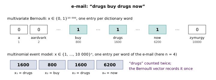
22:34 The alternative represents an e-mail of words as a vector of length , whose th entry is the dictionary index of the th word: here . The length now varies from e-mail to e-mail, for the th training example, which also answers a property of text Ng points out — e-mails can be five words long or a thousand, and the binary representation forces both into one fixed-length vector.
23:57 The names are, in Ng’s words, “very confusing, very horrible names”, but they are the ones the field uses. The binary model is the multivariate Bernoulli event model — 10,000 coin tosses, one per word, each deciding whether that word appears. The new one is the multinomial event model. 24:49 Ng credits the naming to his friend Andrew McCallum, and the paper that compares the two, by McCallum and Nigam, says it set out to clear up exactly this confusion.
25:12 The generative story is that the sender first decides spam or not, with probability , and then draws each word of the e-mail independently from one distribution over the vocabulary that depends on the class. So
which looks identical to lecture 5’s naive Bayes and means something different: the product now runs over the words of the e-mail rather than over the dictionary, and each factor is a multinomial over 10,000 outcomes rather than a coin toss. The parameters are and , the chance that a word in a class- e-mail is word . 28:05 Ng puts a question to the room — “the chance of word blank being blank” — and the answer, any position being word , exposes the hidden assumption: the distribution does not depend on . The first word of a spam e-mail is “drugs” with the same probability as the third, which is why does not appear on the left-hand side.
29:41 The maximum likelihood estimates are again counts, now over word occurrences instead of e-mails, and with Laplace smoothing they are
In English: pool every word of every non-spam e-mail, and ask what fraction of them are word . If the non-spam e-mails contain 100,000 words in all and “drugs” is 200 of them, the unsmoothed estimate is . 31:59 Ng asks the room what to add to the denominator for smoothing, and the answer is the number of values can take: the vocabulary size, 10,000, not two.
33:44 A student asks what to do with a word that is not in the dictionary at all. Either drop it, or map every out-of-vocabulary word to one special token, conventionally UNK, which then gets a probability like any other word. The second keeps the information that the e-mail contained rare words, which can itself be evidence.
The multinomial model is still a linear classifier, now in word counts. Taking the log of Bayes’ rule, the log-odds of spam is
where is the number of times word occurs in the e-mail. The generator confirms this against Bayes’ rule on 200 random e-mails. A repeated word now adds its weight once per occurrence, which is precisely the information the Bernoulli model discarded. McCallum and Nigam’s comparison on five corpora found the Bernoulli model competitive with small vocabularies and the multinomial model usually better with large ones, averaging a 27 percent reduction in error — “much better”, as the lecture puts it, for the typical text problem.
cs229-notes2, section 2.1, gives Laplace smoothing for the binary naive Bayes model; section 2.2 writes out the multinomial event model’s likelihood and both smoothed estimates.
6.4 Build something quick and dirty first
35:26 Naive Bayes is rarely the most accurate choice — logistic regression usually beats it — so the question is what it is for. Ng’s answer is a piece of working advice that appears in no PDF. 36:55 If your goal is to make a learning algorithm work for an application, rather than to invent a new algorithm, start by implementing something simple and fast, train it, look at how it fails, and let the failures decide what to build next. 38:11 His analogy is software: nobody writes 10,000 lines of code and compiles them for the first time at the end; you write a module, test it, and build up. A complicated learning system designed in full before any of it runs is the same mistake.
39:07 The spam filter shows why. Ng started a conference on e-mail and anti-spam, and his example list of promising ideas is long. Spammers misspell deliberately — “m0rtgage”, or the word broken up with slashes — so a filter keyed to words sees an unknown token where a person sees “mortgage”; one of his students published on mapping such spellings back to words. Spammers spoof headers to hide where mail came from. You could fetch the URLs in an e-mail and analyse the pages behind them. 40:59 Each of these is three to six months of work, and at the start you cannot know which one matters. So build the crude filter, then read the e-mails it gets wrong. If many of them are deliberate misspellings, you now have evidence that the misspelling problem is worth months; if few are, “don’t bother” — and you have saved the months. This is error analysis, which the course returns to later.
42:06 That is the niche for naive Bayes and GDA. Neither will give the best accuracy; logistic regression, SVMs and neural networks almost always do better. But both are non-iterative — counting, or computing means and covariances — and short to write, so they are a fast way to get the first system running. Ng’s advice for course projects follows: do not spend weeks designing; get a data set and apply something simple, logistic regression or naive Bayes rather than a neural network, and go from there.
44:26 A student points to a weakness of the word features themselves: “mother” and “father”, or “one” and “two”, are entirely unrelated indices to naive Bayes, which has no way to know that similar words should behave similarly. Ng agrees and names the fix from neural networks, word embeddings, which represent each word by a vector learned so that related words land close together. Because the embedding comes with that knowledge built in, a classifier built on it needs fewer labelled examples. The course leaves the topic to CS230 and CS224N.
6.5 Why support vector machines
46:22 The SVM enters with a picture: two classes in the plane whose boundary is clearly curved. Logistic regression and GDA, as they stand, draw straight lines. 47:06 You can get a curve out of logistic regression by inventing features — map to and fit the same linear model to — and with the quadratic terms the boundary can become an ellipse (Figure 6.2). The generator fits both models to the same data: on the raw features logistic regression misclassifies a third of the training set, with the quadratic terms 12 percent.
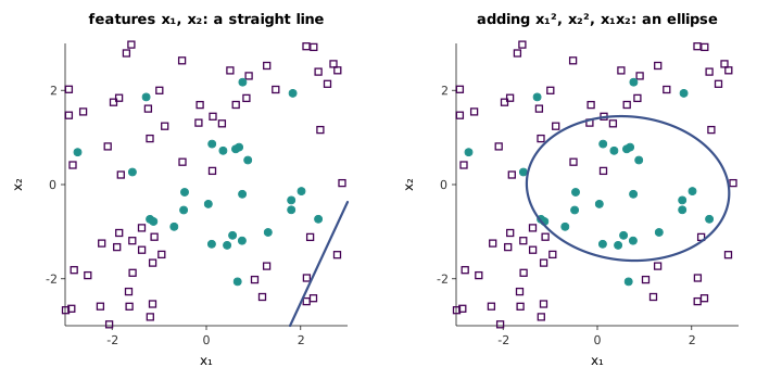
48:05 The trouble is choosing the features. An ellipse needs quadratic terms; Ng admits he would not know which features produce the irregular boundary he drew, and nobody wants to guess between and . The SVM’s promise is to map into a much higher-dimensional feature space — 51:15 hundreds of thousands of dimensions, or infinitely many — and fit a linear classifier there, which is non-linear back in the original space, without anyone choosing the features by hand. That is the kernel idea of lecture 7.
48:48 Ng’s other reason is practical. The SVM is “turnkey”: mature software solves its optimisation problem reliably, without a learning rate to tune or a convergence to babysit. He is explicit that for many problems neural networks are now more effective, and equally explicit that practice uses a much wider set of tools than the press coverage of deep learning suggests.
49:57 The road map has three stages: the optimal margin classifier for data that a straight line can separate, which this lecture starts; kernels, which run it in huge feature spaces; and a modification for data that cannot be separated. The first stage needs two definitions of margin.
6.6 The functional margin
54:50 Ng motivates the margin with logistic regression. The classifier predicts when , but a correct prediction can be confident or marginal. If we would like , so that is close to ; if we would like . A classifier for which both hold on every example is correct and confident.
1:00:02 The SVM changes notation to make the algebra cleaner. Labels are , the hypothesis outputs a hard instead of a probability, if and otherwise, and the intercept is pulled out of the parameter vector: , with playing the role of and of , and no convention.
1:03:36 The functional margin of the hyperplane with respect to the example is
The label folds the two hopes into one: if we want large and positive, if large and negative, and either way we want large. 1:06:30 Its sign alone already says something: exactly when the example is classified correctly. 1:07:46 For the whole training set, the SVM takes the worst case, — how well the classifier does on the example it does worst on. That is a harsh notion, and it makes sense for now only because this lecture assumes the data are linearly separable.
1:09:01 The functional margin has a flaw Ng calls cheating. Multiply and by , or , and every multiplies by the same factor, yet the boundary is the same line and every prediction is unchanged (the generator checks this for factors of , and , Ng’s choices). So “make the functional margin large” is not a goal at all: any separating classifier achieves an arbitrarily large one. 1:10:00 The fix is to normalise — require , or equivalently divide and by — and the freedom to rescale without changing the classifier turns out to be useful later rather than only a nuisance.
6.7 The geometric margin
1:11:29 The geometric margin is the normalised version, and it has a picture. The line splits the plane into the half where the classifier predicts and the half where it predicts , and the vector is perpendicular to the line, pointing into the positive half. 1:12:33 For a correctly classified positive example , the geometric margin is its Euclidean distance to the line: the length of the segment from to the nearest point on the boundary (Figure 6.3).
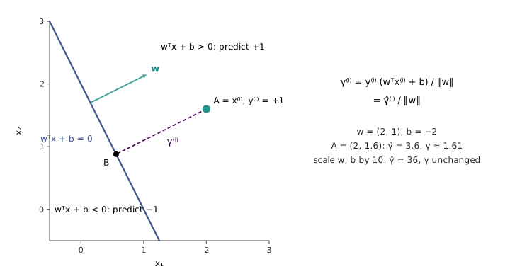
1:13:49 Ng states the formula and leaves the derivation to the notes; it is short enough to give. is moved back along the unit normal by the distance , so , and lies on the line, so . Solving gives for a positive example, and including the label makes it hold for negative ones too:
For the point in Figure 6.3, the functional margin is and the geometric margin ; multiply and by ten and the functional margin becomes while the geometric margin stays at . The geometric margin is the functional margin with the cheat removed. The generator checks Equation 6.5 against an explicit projection onto the hyperplane for 500 random hyperplanes and points in three dimensions. 1:15:23 As before, the training set’s geometric margin is the worst case, .
6.8 The optimal margin classifier
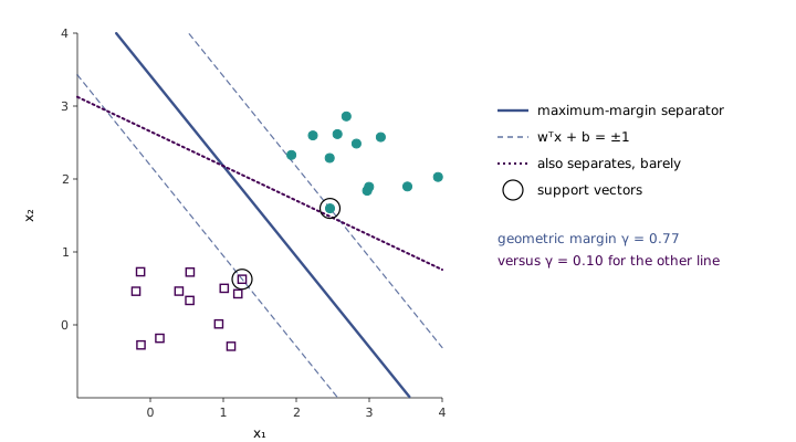
58:15 Ng drew the motivating picture well before the definitions. Two lines both separate a training set perfectly; one passes close to a few of the examples, the other keeps a wide berth from both classes, and the second “looks much better”. The geometric margin is what “looks better” means: the first line’s worst example is barely on the right side, the second line’s is far from it (Figure 6.4).
1:16:28 The optimal margin classifier chooses and to maximise the geometric margin of the training set. 1:17:59 Ng poses it as a problem in three unknowns, , and :
Every example must have geometric margin at least , and is pushed as high as the constraints allow, so at the optimum equals the worst example’s margin and that worst margin is as large as it can be.
1:19:03 In this form the problem is not convex, so there is no guarantee that a local method finds the global optimum. 1:19:13 Ng states, and leaves the steps to lecture 7 and the notes, that a few rewrites turn it into an equivalent convex problem: minimise subject to every functional margin being at least . His one-line intuition is that the margin is the functional margin divided by , so a smaller means a smaller divisor and a larger geometric margin. Off-the-shelf solvers handle the convex form, and for separable data its solution is the optimal margin classifier — “really a baby SVM”, which kernels will grow up.
The solution has a property the picture already shows. In Figure 6.4 only two examples touch the dashed lines; they are the support vectors, and the separator depends on them alone. The generator finds this separator in two independent ways. It searches over directions for the one that leaves the widest gap between the classes, and then checks the result against the optimality conditions of the convex problem: every functional margin is at least , the two closest examples have functional margin exactly , and over those two examples alone, with both . That last fact — the solution is built from a few training examples — is where lecture 7 begins.
cs229-notes3, sections 1–4, defines the functional and geometric margins with the same notation and gives the full chain of rewrites from Equation 6.6 to the convex quadratic program.