1 Introduction
Lecture 1
machine learning, supervised learning, unsupervised learning, reinforcement learning, CS229 introduction
Lecture video: Lecture 1: Introduction · 1:15:20
Based on the lecture by Andrew Ng — CS229, Stanford University, Autumn 2018.
The first lecture of CS229 does two things. It places the course among Stanford’s other machine-learning courses, and it draws, in about forty minutes at the board, the map the remaining nineteen lectures fill in: learning from labelled examples, learning to apply learning algorithms well, deep learning, learning from data with no labels, and learning from reward. No algorithm is derived. What the lecture supplies instead is the set of pictures — a scatter of house prices, a row of noughts and crosses, two clouds of unlabelled points — that every later derivation is drawn on top of, and it is worth having them clearly in mind before the mathematics arrives.
1.1 What the course assumes
10:22 The stated prerequisites are modest on paper: familiarity with basic probability and statistics, basic linear algebra, and enough programming to write non-trivial code. In 2018 the assignments moved from MATLAB and Octave to Python and NumPy, which Ng presented as following the field rather than leading it.
The more useful guidance came from a question at 28:37 about how CS229 differs from CS229A and CS230. Ng’s answer was not a list of topics but a statement about depth. CS229A, taught as a flipped classroom built on his online course, covers a similarly broad set of algorithms with much less mathematics; CS230 is narrower, deep learning only, and also more applied. CS229 is the one that derives things, and he was candid that the derivations make it a heavy course. His advice to anyone unsure whether they were ready was to take CS229A first. He also pointed out that the three overlap less than their titles suggest — students who took two at once saw the same algorithms from different angles rather than the same lectures twice — and closed with the remark that frames the rest of the course: AI is larger than machine learning, and machine learning is larger than deep learning.
1.2 Two definitions
36:17 Ng offers two definitions of machine learning, an informal one and an operational one.
The informal one is usually credited to Arthur Samuel: machine learning is the field of study that gives computers the ability to learn without being explicitly programmed. That exact sentence does not appear in Samuel’s paper, Some Studies in Machine Learning Using the Game of Checkers (1959), and is better read as a later paraphrase of it. Samuel’s own wording describes programming a computer “to behave in a way which, if done by human beings or animals, would be described as involving the process of learning”. The result the lecture attaches to it is in the paper, and it is what made the work famous. Samuel’s program, given the rules of checkers and a list of board features with unknown weights, learned to play a better game than Samuel himself, partly by playing against a copy of itself and keeping whichever set of weights won. The abstract puts the training time at eight to ten hours of machine-playing time.
Ng’s point about this is historical. At the time the open question was whether a computer could do anything it had not been explicitly told to do, and a program that beat its own author was a direct answer. Today it is routine for a learning algorithm to outperform people on a narrow task — a particular kind of speech recognition, or Go given enormous amounts of computation and self-play — and he stresses the word narrow. Samuel’s checkers player was among the first cases of that pattern.
The operational definition is Tom Mitchell’s, from his 1997 textbook Machine Learning, which calls something a well-posed learning problem when three things are named. A program learns from experience with respect to a task and a performance measure if its performance on , as measured by , improves with . 38:43 Applied to checkers, is playing the game, is the large number of games the program plays against itself, and is the probability of winning its next game against a new opponent. The value of the definition is that it forces all three to be stated. A good deal of what goes wrong in applied machine learning, which the course returns to in its lectures on strategy, is a project where one of them was never pinned down: the team is measuring a that does not track the they care about, or gathering an that does not resemble the situations the system will face.
1.3 Supervised learning: regression
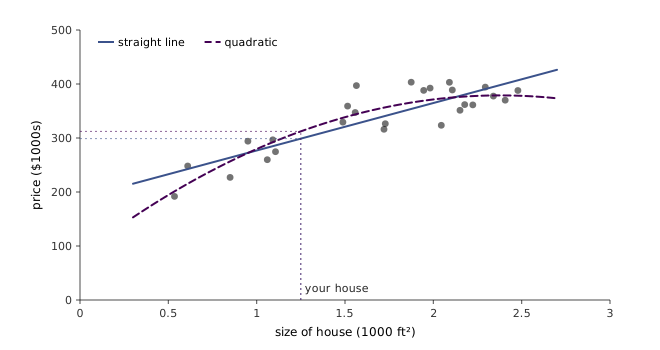
40:12 The most widely used kind of machine learning, and the subject of the first third of the course, is supervised learning. Ng introduces it with the example the next lecture formalises. Plot the size of each house in a dataset on the horizontal axis and its sale price on the vertical, call the first and the second , and ask for the relationship between them. If you own a house of 1,250 square feet and want to know what to ask for it, one answer is to fit a straight line to the data and read the price off the line above 1,250.
figures/01-introduction/make_diagrams.py.
That is the whole shape of supervised learning. You are given a training set of inputs paired with the correct outputs , and the job is to learn a mapping from to good enough to apply to an you have not seen. The problem is called regression when is continuous. Prices are rounded to the cent and so are not literally real numbers, Ng notes, but nobody prices a house at million dollars and for every practical purpose they are continuous.
A straight line is close to the simplest learning algorithm there is, and Figure 1.1 shows why it is not the only candidate. A quadratic follows the flattening of prices at the top end and has lower error on the training points (an RMSE of 25.4 against 29.6 on this data). That comparison cannot settle the question, though. A quadratic can never fit its training data worse than a line, because every line is a quadratic whose coefficient is zero, and this particular quadratic peaks at about 2,400 square feet and predicts that every house larger than that is worth less. How to choose between models — the line, the quadratic, or something richer, whether by hand or automatically — is one of the questions Ng flags as recurring all quarter. It becomes the bias–variance discussion of lecture 8.
1.4 Supervised learning: classification
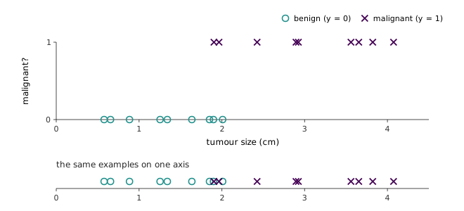
43:04 The second example comes from a medical problem some of Ng’s collaborators worked on: deciding from a breast tumour’s size whether it is malignant or benign. Plot size on the horizontal axis and, on the vertical, for malignant and for benign. When a new patient arrives with a tumour of a given size, the learning algorithm should say how likely it is to be malignant. Because now takes one of a small number of discrete values, this is classification. With two values it is binary classification, and with, say, five types of cancer it is still classification, just with five classes.
45:37 Ng then redraws the same data in a form the course uses from then on. Every example is pushed up onto a single horizontal line, and the label is carried by the symbol rather than by the height: a nought for a negative example (), a cross for a positive one (). Nothing is lost — Figure 1.2 shows both views of identical data — but the second frees the vertical axis to hold a second input.
figures/01-introduction/make_diagrams.py.
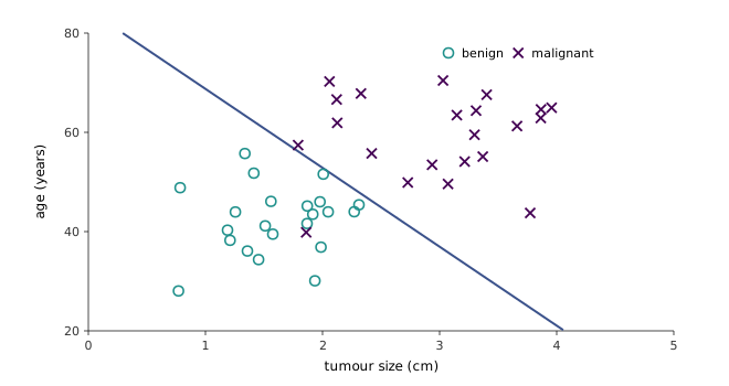
47:07 That is the step he takes next. Real problems rarely give you one number to predict another; with the patient’s age as a second feature, becomes a two-dimensional vector of tumour size and age, and each example becomes a nought or a cross in the plane. The task is now to separate the two kinds of mark, and the algorithm the course reaches for first draws a straight line between them. That algorithm is logistic regression, taken up in lecture 3, and it is what fitted the boundary in Figure 1.3.
figures/01-introduction/make_diagrams.py.
1.5 More features than you can draw
48:41 The two-feature picture is a teaching device. The group Ng describes used many more measurements of each tumour: clump thickness, uniformity of cell size, uniformity of cell shape, marginal adhesion. Those are attributes of the Wisconsin breast cancer data (Breast Cancer Wisconsin (Original)), which scores each of nine cytological features on a scale of one to ten. Nine dimensions cannot be plotted. The algorithms of the coming weeks are therefore written for an input vector of any length, and the board pictures are the case drawn to build intuition.
50:11 Ng then makes the remark of the lecture that most deserves a second look. The support vector machine, he says, can represent each patient not by two numbers or a million, but by an infinite list of features. His question is the one a reader should ask: a computer cannot store infinitely many numbers, so how can that work?
The answer, which lecture 7 develops, is that the algorithm never needs the features themselves. It only ever needs inner products between pairs of feature vectors, and for well-chosen feature maps that inner product has a closed form. A one-dimensional example shows it. Map a scalar to the infinite vector
The inner product of two such vectors is a power series that sums exactly:
The left-hand side is an inner product in infinitely many dimensions; the right-hand side is one subtraction and one exponential. The generator for this chapter checks the identity numerically. For and , the first five coordinates of already match the exact value to within , and ten match it to about . A function like the right-hand side of Equation 1.2 is called a kernel, and this one is the Gaussian kernel. The SVM is written so that features appear only inside such inner products, and that is the whole of the trick Ng is foreshadowing.
1.6 Learning to steer: ALVINN
52:05 The idea underneath all of this, Ng says, is that during training the algorithm sees inputs together with their labels , and its job is to find a mapping that produces the right for a new . To show how far that idea goes, he plays an old video of Dean Pomerleau’s ALVINN at Carnegie Mellon, a neural network that learned to steer a vehicle.
The set-up is supervised learning with a human as the labeller. While a person drives, the vehicle repeatedly digitises the camera image of the road ahead, downsampled to a small greyscale picture, and records the steering direction the driver chose at that moment. The image is and the driver’s steering is . On screen the label is a bright blob on a bar, a little left of centre when the driver is turning slightly left, and the network’s output is drawn on a second bar beneath it. At the start of training the network’s output is a grey smear across the whole bar, its way of saying it has no idea which way to steer. As training proceeds the smear contracts to a sharp blob that tracks the driver’s. Then the driver takes their hands off the wheel and the network steers. A later version in the video trains separate networks for one-lane and two-lane roads, with an arbitrator choosing between them, and switches from one to the other as the road changes.
Ng is clear that this is not how self-driving cars are built now. The example is in the lecture because it is a supervised learning problem whose labels cost nothing except someone driving, and because the techniques that make it work — gradient descent and backpropagation — are the ones the course teaches in its first weeks and in lectures 10 and 11.
1.7 Machine learning strategy
58:01 The second area of the course, which the class notes file under learning theory, is what Ng calls machine learning strategy, and his motivation for it is drawn from practice rather than from theory. Visiting machine-learning teams at large technology companies, he finds an enormous difference in how effectively two teams apply the same algorithm. The failure he describes is a team that has spent six months on an approach, where a look at the data shows that it was never going to work, and that could have been seen at the start.
The decisions behind that are the everyday ones: whether to collect more data and which data, whether to try a different algorithm, whether to rent faster GPUs and train for longer, which architecture to use. 1:01:08 A learning algorithm, he says, almost never works the first time, so what separates teams is how they debug. His two analogies are both about debugging by principle rather than by reflex. One is a friend who dealt with compiler errors by deleting every line that had one. The other is the difference between an inexperienced engineer who starts optimising code at once and an experienced one who runs a profiler first and changes only the bottleneck. The aim is to turn what has been “black magic”, tribal knowledge held by people with decades of experience, into an engineering discipline that can be taught. That material comes in lecture 8, the learning-theory discussion section, and lecture 12 on debugging and error analysis.
Deep learning is the third area. Ng describes it as the part of the field moving fastest and treats it as one tool among many. CS229 covers enough to train a neural network from scratch in lectures 10 and 11, and leaves the depth to CS230.
1.8 Unsupervised learning
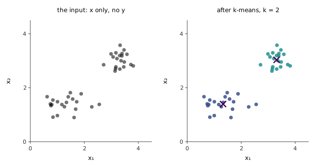
1:04:57 Ng introduces unsupervised learning by redrawing the classification picture and deleting the labels. You are given only the inputs , no , and asked to find interesting structure in them. In the data on the board the structure is visible at a glance — two clusters — and an algorithm the course covers, k-means clustering, finds it. Figure 1.4 runs that algorithm on synthetic points like the board’s. Starting from two arbitrary points as centres, it reaches a stable split in three rounds of reassignment.
figures/01-introduction/make_diagrams.py.
The applications Ng lists show how much of clustering is grouping things that nobody has named. Google News gathers thousands of articles a day by different reporters into a single story, such as the BP oil-well spill. Genetic microarray data group individuals by shared characteristics. Clustering groups machines in a data centre by related workloads, finds the cohesive communities in a social network, and splits a customer database into market segments that can be addressed separately. A colleague of his has used it to group galaxies in astronomical data.
1:08:12 A student asked the natural question: is unsupervised learning just clustering? It is not. Unsupervised learning means any use of unlabelled data to find something interesting, and clustering is one instance. Ng’s second example is the cocktail party problem. Put several microphones in a room where several people are talking at once. Each microphone records an overlapping mixture of every voice, and the task is to recover each speaker’s voice cleanly. Nothing labels which sound came from whom, which is what makes the problem unsupervised. The algorithm that solves it, independent component analysis, is in lectures 15 and 16 and is a programming exercise later in the course. His third example is text. From unlabelled text alone, word representations can be learned that capture analogies such as man is to woman as king is to queen and Tokyo is to Japan as Washington, D.C. is to the United States, the result popularised by Mikolov et al. (2013).
He also offered a judgement on the economics. Most of the value machine learning was creating in 2018 came from supervised learning, while unsupervised learning had important uses and was where much of the research frontier lay.
1.9 Reinforcement learning
1:11:19 The fifth area starts from a problem that defeats supervised learning: if you were handed the keys to Stanford’s autonomous helicopter, how would you write a program to fly it? The difficulty is that nobody knows the optimal way to move a helicopter’s two control sticks, so there is no to label each state with, and no expert whose every action is worth imitating as ALVINN imitated its driver.
1:12:18 Ng’s analogy is training a dog. You cannot show a dog the optimal way to behave either. You let it do what it wants and say “good dog” when it does something you like and “bad dog” when it does not, and over time it does more of the first and less of the second. Reinforcement learning replaces the label with that signal, called the reward. The helicopter flies however it likes, gets “good helicopter” for an accurate manoeuvre and “bad helicopter” when it crashes, and the algorithm’s job is to find a way of acting that collects more reward over time. The helicopter in the video is the Stanford autonomous helicopter, whose aerobatic flight is described in Abbeel et al., 2006, and a second clip applies the same reward-driven learning to a legged robot dog learning to climb over obstacles.
The best-known successes of reinforcement learning were in games, Atari and AlphaGo. Ng said he was as excited, or more, by its growing traction in robotics and in optimising logistics systems. The course’s last five lectures build it up from Markov decision processes.
1.10 The map of the course
1:11:11 Ng closes the overview with the list of the five areas. They map onto this book as follows.
| Area | What it is about | Lectures |
|---|---|---|
| Supervised learning | learning a mapping from labelled pairs | 2–7, 9 |
| Learning theory and strategy | why learning works, and how to make it work in practice | 8, learning theory, 12 |
| Deep learning | training neural networks | 10–11 |
| Unsupervised learning | finding structure in alone | 13–16 |
| Reinforcement learning | learning to act from a reward signal | 16–20 |
The order is deliberate. Supervised learning comes first because it is where both the mathematics and the economic value are most developed, and every later area borrows its notation. The next chapter starts there, with the house-price scatter of Figure 1.1 and the first algorithm for fitting it.