7 Kernels
Lecture 7
kernel trick, support vector machines, Lagrange duality, representer theorem, Mercer’s theorem, soft margin SVM
Lecture video: Lecture 7: Kernels · 1:20:25
Based on the lecture by Andrew Ng — CS229, Stanford University, Autumn 2018.
A support vector machine is the optimal margin classifier of lecture 6 run in a feature space of enormous, possibly infinite, dimension. That sounds impossible to compute, and the lecture’s argument is a chain of three observations that make it cheap. The optimal is always a weighted sum of the training examples. Once is written that way, the training problem and the prediction rule touch the data only through inner products . And for some very large feature maps , the inner product can be computed directly from and in time proportional to their own dimension — that shortcut is a kernel. Ng calls the SVM one of his favourite algorithms because it is “very turnkey”: the optimisation is convex and good packages solve it. The lecture ends by dropping the assumption that the data are separable and with kernels designed for inputs that are not vectors at all.
7.1 From the largest margin to the smallest
1:13 Lecture 6 posed the optimal margin classifier as: choose , and to maximise , subject to every example having geometric margin at least . 5:31 Ng spends a minute on why that maximises the worst margin. If three examples had geometric margins , and , the set’s margin is , and the only way to raise under the constraints is to raise the margin of whichever example is lowest. Pushing up as far as it goes is the same as maximising .
6:33 The step to a tractable problem uses the freedom that made the functional margin useless in lecture 6. Take and : the boundary crosses the axes at and , and so does the boundary for and , or for and . Because rescaling changes nothing about the classifier, we may pick the scale, and 8:49 the convenient choice is the one that makes the worst functional margin exactly : . Then the geometric margin is , maximising it is minimising , and minimising the smooth has the same solution:
This is a convex quadratic objective under linear constraints — a quadratic program, with one global optimum and reliable solvers. On lecture 6’s example set the solution has , so , the same margin lecture 6’s generator found by searching over directions; the two examples that touch the margin have functional margin exactly and every other example more.
7.2 The representer theorem
10:34 So far has been two- or a hundred-dimensional. The goal is feature vectors with a hundred trillion dimensions, or infinitely many, where cannot even be stored. 11:07 The way through is to assume that is a linear combination of the training examples,
with the labels written in by convention because they make later algebra tidier. 11:57 Ng presents this as an assumption but stresses that it is not one: the representer theorem proves that the optimal always has this form, so nothing is lost. He skips the proof as long and involved and gives two intuitions.
13:11 The first is from gradient descent. Run stochastic gradient descent for logistic regression from . Each update adds a multiple of one training example, (this is the learning rate, unrelated to the above). By induction, is a linear combination of training examples after every step, however many steps you take; 15:22 batch gradient descent is the same, and so is gradient descent on the SVM’s own objective. The generator runs 300 SGD steps in five dimensions on three examples and finds within of the span of those three vectors.
16:09 The second is geometric. 16:50 The vector is perpendicular to the decision boundary: it fixes the boundary’s orientation, and slides the boundary along it. 18:39 Now suppose the inputs have three features but every training example has , so the data lie in the -plane. Then, Ng says, should be — should lie in the space the examples span.
That second intuition is worth sharpening, because as stated it is not true of every separator. With all , the term is zero on every training example, so any value of classifies the training set identically: the generator takes the SVM’s and sets , and every margin constraint still holds. What forces is the objective. A non-zero adds to and buys nothing in the constraints, so the minimum-norm solution drops it. That is the real content of the representer theorem: among all the that fit the data equally well, minimising (or, in general, any loss plus a squared-norm regulariser) picks one in the span of the data.
7.3 Everything is an inner product
20:34 Substitute Equation 7.2 into Equation 7.1. Since , the objective becomes
and the constraints become , where is the inner product. 24:13 The point is where the inputs now appear: nowhere except inside inner products. Whatever the dimension of , the problem is stated in terms of the table of inner products between training examples.
25:14 The form actually solved in practice goes one step further. Ng skips the derivation, which uses Lagrange duality, and writes down the result, the dual optimisation problem:
has dropped out, to be recovered afterwards from any example with . Two facts about Equation 7.3 go beyond the lecture and are worth having. First, it is not merely a simplification of the substituted problem: when there are more examples than dimensions, many different give the same , and the dual picks out particular ones — non-negative, and zero for every example that is not on the margin. Those with are the support vectors. Second, its optimal value equals the primal’s: on lecture 6’s data the generator solves Equation 7.3 by sequential minimal optimisation, the algorithm in the official notes, and finds , with only 2 of the 24 non-zero, and the resulting and agree with lecture 6’s direction search to five decimal places.
27:05 Prediction is an inner product too:
28:20 Once the are stored, both training and prediction need nothing but inner products of inputs — and since most are zero, prediction sums only over the support vectors.
cs229-notes3, section 5, derives Lagrange duality and the KKT conditions, and section 6 applies them to obtain Equation 7.3 and the formula for . The representer theorem, with a proof for general losses, is in the supplementary notes on the representer theorem, section 2.
7.4 The kernel trick
28:42 Ng gives the recipe in four steps. First, write the whole algorithm in terms of inner products . Second, choose a feature map from the original inputs to a higher-dimensional space — 30:12 a house’s floor area could become , or area and bedrooms could become all their products up to some degree. Third, find a way to compute
the kernel function, cheaply. Fourth, replace every in the algorithm by . 32:19 The algorithm is then running on , in the high-dimensional space, without ever forming . Forming it is what would be expensive: Ng has seen problems with a billion features, and even 100,000 makes every vector operation costly.
33:55 A student asks about the no-free-lunch theorem, and Ng’s answer frames why this works at all. The theorem — Wolpert’s form of it for supervised learning shows that, averaged over all possible target functions, no learning algorithm has lower off-training-set error than any other — says that in the worst case learning does not work. Ng finds it less useful than fascinating, because the problems we meet are not drawn adversarially: “the universe is not that hostile toward us”, and an inductive bias such as “the boundary is smooth in some feature space” tends to pay off.
7.5 Polynomial kernels
34:42 The first example shows the saving. Let and let list every product — for , the nine terms , duplicates included. 35:38 So : with that is features, and computing explicitly takes order time. 37:18 But
and the left-hand side takes order time: one inner product of -vectors, then one squaring. The middle expression is the explicit computation — march down both lists of products, multiply, add — and the identity says that the cheap computation gives the same number.
41:11 Adding a constant, , corresponds to appending the first-degree terms and a constant to the features: now also contains and . The constant sets the relative weight of the linear terms against the quadratic ones. 42:29 More generally, is still order to compute and corresponds to a containing every monomial of degree up to — terms like or when — each with a weight that involves and a multinomial coefficient. The generator builds these explicit feature vectors for and and confirms that their inner product equals the kernel on 200 random pairs.
42:56 Ng gives the number of distinct monomials as , which the generator confirms by enumeration, and then glosses it as “roughly , very roughly”. The binomial coefficient is the right count; the gloss is high by about a factor of . For and , while , a ratio of . The point survives — the feature space grows like , astronomically, while the kernel costs order for every .
44:23 This is what Ng means by the SVM: the optimal margin classifier plus the kernel trick. Choose a kernel, solve Equation 7.3 with in place of the inner products, and predict with Equation 7.4 likewise; the computation scales with the dimension of , not of . 45:51 A student asks whether a kernel belongs to one feature map. Essentially yes: up to trivial changes such as permuting the features, which leave every inner product unchanged, a different feature map needs a different kernel.
7.6 Seeing the lift
47:09 To show what this does geometrically, Ng plays a short visualisation by Udi Aharoni. Red and blue points in the plane cannot be separated by a line; a feature map lifts them into three dimensions, where a plane separates them; and the plane, viewed back in the original plane, cuts out an ellipse. Figure 7.1 does the same thing one dimension lower, so it fits on a page. The positives sit between the negatives on a line, so no single threshold separates them. Map each to and the points land on a parabola, where the SVM finds a straight line; pulled back to the original line, that straight line becomes the two thresholds and .
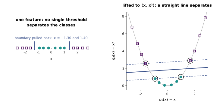
49:10 The boundary is linear in a high-dimensional space and very non-linear in the original one. 49:27 A student asks whether the data must be linearly separable in that high-dimensional space; so far the derivation has pretended so, and the soft margin below removes the assumption.
7.7 Which functions are kernels
50:02 Ng’s working intuition is that a kernel measures similarity. An inner product is large when two vectors point the same way and small when they point in unrelated directions, so should be large when and are alike and small when they are not. 51:19 By that standard, here is a function pulled “out of the air”:
close to when and are near each other and close to when they are far apart. 52:13 Can it be used? Only if some makes ; the whole derivation assumed so, and a without such a breaks it — the optimisation problem may no longer correspond to any classifier at all.
53:01 One necessary condition is immediate: . 53:27 A stronger one comes from taking any points and forming the kernel matrix (or Gram matrix) . For any vector ,
so a valid kernel always produces a positive semidefinite kernel matrix (and a symmetric one, since inner products are). 57:21 Mercer’s theorem says the converse holds too: is a valid kernel if and only if, for every finite set of points, the kernel matrix is symmetric positive semidefinite. Ng proves only the direction above and states the other.
The similarity intuition is a good guide but not a test, and the gap is easy to fall into. “Two points are similar if they are within 1.5 of each other” sounds like a reasonable similarity, . At the three points its kernel matrix has eigenvalues , and ; the vector gives . No feature map produces that matrix, so it is not a kernel, and the SVM built on it can fail to be a convex problem. The generator checks this alongside the Gaussian kernel, whose kernel matrix on 25 random points has every eigenvalue non-negative.
59:13 Equation 7.7 is valid, and it is called the Gaussian kernel. 59:36 The most widely used kernel is in fact the linear kernel, with — the SVM with no feature map at all — and the Gaussian is next. 1:00:11 Its feature space is infinite-dimensional, and Ng describes it as containing every monomial, of every degree, with the high-degree ones given smaller weight. That can be made exact in one dimension:
The weight on the degree- feature falls like , which is the “smaller weighting” in concrete form. The generator truncates the sum: with , on sixteen pairs of inputs drawn from , three features reproduce the kernel to within , twelve to within , and twenty to rounding error.
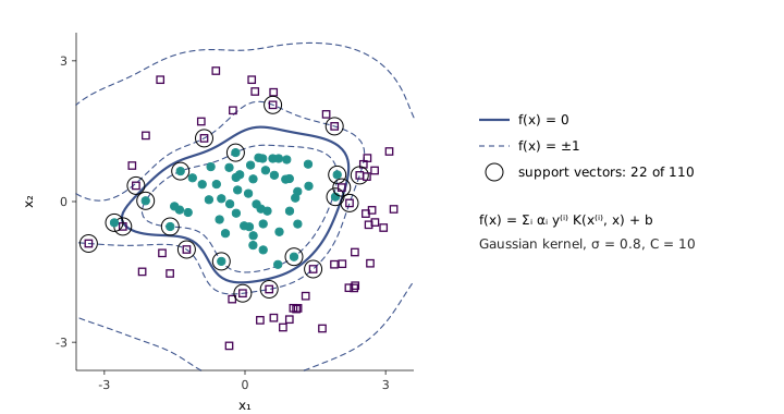
Figure 7.2 shows the Gaussian kernel at work on data no polynomial of low degree separates cleanly: a disc of one class inside a ring of the other. The decision function is a sum of bumps centred on the support vectors, 22 of the 110 examples, and its zero level set is the closed curve between the classes.
7.8 Kernelising other algorithms
1:01:20 The kernel trick is not specific to the SVM. Any algorithm that can be written in terms of inner products of inputs can be kernelised, and Ng lists linear regression, logistic regression, every generalised linear model, the perceptron (which the problem sets kernelise) and, later in the course, principal components analysis. Linear regression in an infinite-dimensional feature space is a perfectly well-defined computation. 1:03:07 In practice, though, the trick is applied overwhelmingly to SVMs and much less often elsewhere.
1:01:26 Ng credits the popularisation to Vladimir Vapnik and Corinna Cortes. The history is slightly split between two papers. The kernelised maximum-margin classifier was introduced by Boser, Guyon and Vapnik in 1992; Cortes and Vapnik’s “Support-vector networks” of 1995 added the soft margin of the next section.
7.9 The soft margin
1:04:07 Mapping to a high-dimensional space makes data much more separable, but a separating boundary is not always wanted. If the data are slightly noisy, a boundary that classifies every training example correctly may be contorting itself around a few mislabelled ones. 1:05:17 The -norm soft margin SVM relaxes the constraint that every functional margin be at least , allowing a slack per example and charging for it:
1:06:49 Recall that a positive functional margin means a correct prediction; the hard-margin SVM demands more, a functional margin of at least . A slack of lets example get away with functional margin ; a slack above lets it be misclassified. At the optimum each slack is as small as its constraint allows, , so Equation 7.8 is the same as minimising plus times the hinge loss summed over the training set — a form worth recognising, since it puts the SVM beside logistic regression as a regularised loss. 1:07:55 The examples on the margin have functional margin exactly , Ng notes, because otherwise the line could be moved to widen the margin; examples further away have larger ones.
1:08:59 His second reason for the soft margin is robustness. The hard-margin classifier maximises the worst-case margin, so a single outlier — technically leaving the data separable — can swing the boundary dramatically. Figure 7.3 measures this on lecture 6’s data with one positive example added near the negatives. The hard-margin normal turns by to squeeze past the outlier and the margin shrinks from to . With , adding the same outlier turns the soft-margin boundary by under ; the outlier simply sits on the wrong side, with slack .
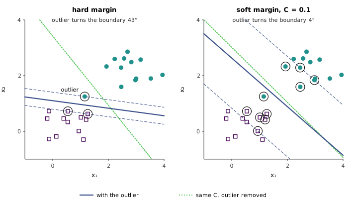
How much protection the soft margin gives depends on , which is the part to take away from the figure. With on the same data the outlier still turns the boundary by : the slack is so expensive that the solution prefers to move. trades the width of the margin against the training errors it will tolerate, and 1:12:58 choosing it is a bias–variance question that lecture 8 takes up.
1:11:34 Repeating the dual derivation for Equation 7.8 changes exactly one thing: the constraint becomes the box . The generator checks the consequences on its solution, which are the optimality conditions in the notes: examples with sit exactly on the margin, every example with positive slack has , and examples beyond the margin have . 1:12:19 Ng’s practical remark is that in the early days of SVMs solving this problem was itself a research worry, much as matrix inversion once was; today’s packages solve it and you need not think about it. The generator’s solver is a version of sequential minimal optimisation, the coordinate method of the official notes, which updates two at a time so that stays satisfied.
cs229-notes3, section 8, derives the dual of the soft-margin problem and its KKT conditions, and section 9 presents the SMO algorithm, including the closed-form update for a pair of under the box constraint.
7.10 Kernels for inputs that are not vectors
1:13:39 In practice the polynomial kernel works well, and Ng now calls the Gaussian kernel the one most used; earlier he gave that place to the linear kernel, and between them the two are the usual first choices. 1:14:05 One of the early proof points for SVMs was handwritten digit recognition: unroll an image into a vector of pixel intensities and train an SVM on it. On the classic MNIST benchmark this was, in Ng’s words, a very surprising result, and polynomial-kernel SVMs appear beside the convolutional networks of the time in the comparison of classifiers by LeCun et al. 1:15:07 Ng’s summary is that SVMs were for a time the best algorithm on it, with convolutional networks pulling ahead in more recent years.
1:15:25 Much of the inventive work on SVMs, Ng says, has gone into designing kernels, and his example is a protein classifier. A protein is a variable-length sequence of amino acids, of which there are 20 (Ng uses the letters A to Z on the board for convenience). 1:17:01 One feature vector for a sequence counts every possible run of four amino acids — how many times AAAA occurs, then AAAB, and so on to the end of the list — so that has entries (with Ng’s 26 letters it would be 456,976). 1:18:20 Writing it out is expensive, but can be computed directly from the two sequences. Ng describes a dynamic programme reminiscent of Knuth–Morris–Pratt string matching; the kernel as published, the spectrum kernel of Leslie, Eskin and Noble, builds a suffix tree and computes it in time linear in the two sequences’ lengths. Only the four-letter runs that actually occur contribute, so a dictionary of counts per sequence is already enough, and the generator confirms that this gives the same number as the explicit 160,000-dimensional inner product.
1:19:35 If the inputs are histograms — the demographic make-up of two countries, say — one kernel sums the bin-by-bin minimum of the two histograms, , a direct measure of their overlap. It is a valid kernel on non-negative histograms, and the proof is one line: , an inner product of two indicator functions. The generator’s kernel matrix on twenty random histograms has, as it must, no negative eigenvalue. The general lesson is the recipe of the kernel trick read backwards: for an unusual kind of input, ask what similarity you would want between two examples, then make sure it is an inner product in some space, and the SVM machinery applies unchanged.