8 Data Splits, Models and Cross-Validation
Lecture 8
bias and variance, overfitting, regularization, cross-validation, train/dev/test split, feature selection
Lecture video: Lecture 8: Data Splits, Models and Cross-Validation · 1:23:26
Based on the lecture by Andrew Ng — CS229, Stanford University, Autumn 2018.
Every learning algorithm so far has come with a knob — the degree of a polynomial, the bandwidth of locally weighted regression, the constant of the soft-margin SVM — and this lecture is about how to set it. The answer has two parts. The first is a diagnosis: a model that is too simple underfits, which Ng calls high bias, and a model that is too flexible overfits, which he calls high variance. The second is a procedure: never judge the knob by training error, because training error always prefers the most flexible model; judge it on data the model was not fitted to, held out once (a dev set) or in rotation (cross-validation). Between the two sits regularisation, the one-line change Ng says he uses more often than almost any other technique, which lets a large model behave like a small one.
Ng opens by saying that bias and variance is “easy to learn, hard to master”: former PhD students of his report that their understanding of it kept deepening for years after the course. The formal learning theory that used to accompany it — error decomposition, uniform convergence, VC dimension — has moved to the Friday discussion section, which has its own chapter. This lecture keeps the working concepts.
8.1 Bias and variance
4:53 Ng draws the same six houses three times, size against price, with prices that rise and then level off. A straight line, , catches the trend but not the bend. A quadratic follows the data well. A fifth-order polynomial has six parameters for six points, so it passes through every one of them exactly — and is plainly a worse model of house prices than the quadratic, wiggling between the points and swinging off wildly beyond the outermost ones.
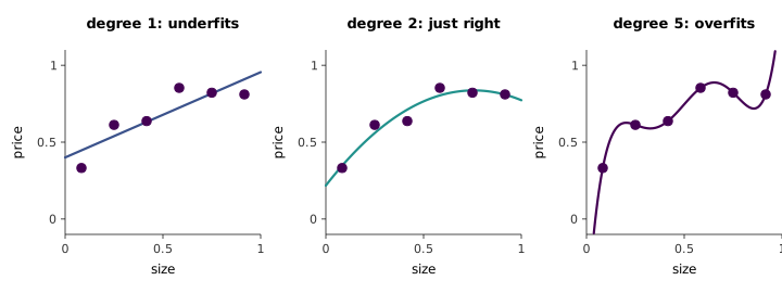
7:04 The line underfits, and Ng says it has high bias. The word has nothing to do with bias in the social sense; it means that the algorithm arrived with a strong preconception — that price is linear in size — and that the preconception is false, so no amount of data will talk it out of the wrong shape. 8:04 The fifth-order polynomial overfits, and has high variance. The name comes from a thought experiment Ng returns to several times: suppose a friend collects their own six houses, from the same market, with slightly different noise. The quadratic fitted to the friend’s data will look much like yours. The fifth-order polynomial will be some completely different curve, because it is fitting the noise, and the noise is what changed.
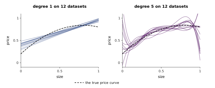
That thought experiment is easy to run, and Figure 8.2 runs it twelve times. The straight lines agree with one another and are all wrong in the same way; that shared error is the bias. The quintics agree only where the data pin them down and scatter everywhere else; that spread is the variance. Averaged over 4,000 friends, the linear fit at the middle of the range misses the true price by (it sits below the bend) with a standard deviation across datasets of only ; the quadratic is unbiased to three decimals with standard deviation . Near the small end of the range, at , the quintic is unbiased too, but its standard deviation is — five times the quadratic’s and larger than most house prices on the plot.
10:06 Classification has the same three regimes. Logistic regression on the raw features draws a straight boundary through data that clearly want a curve; with a handful of hand-chosen features such as , , it draws a sensible curve; with a great many features, or an SVM with a rich kernel, it can draw a contorted boundary that classifies every training example correctly and generalises poorly.
9:30 The reason this matters is practical. Ng’s workflow is to train something quick and dirty first, because a learning algorithm “almost never works the first time”, and then to ask whether it is suffering from bias or from variance, since the remedies for the two are different and often opposite. The diagnostics come in lecture 12. Here the lecture turns to the most common remedy for variance.
27:40 A student asks whether “underfit” and “high bias”, “overfit” and “high variance”, are just synonyms. To a first approximation, Ng says, yes. The exception he flags is a model that has both problems at once: very complex, and still not fitting the data well — a contorted boundary that misses the obvious structure. It is rarer, but it happens.
8.2 Regularisation
13:56 Take the least-squares objective and add one term:
The second term is the regularisation term, and sets its strength; whether it is written or is a matter of which derivations one wants to come out tidy. It gives the algorithm an incentive to keep the parameters small. That is all there is to implement, and Ng warns against underestimating it on that account: it is “deceptively simple” and one of the techniques he reaches for most.
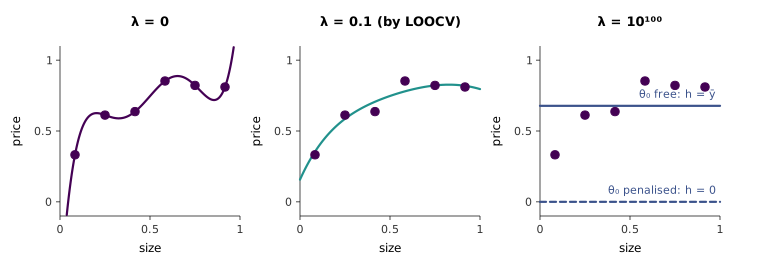
15:17 Put the fifth-order polynomial back on the six houses. With we have the interpolating curve of Figure 8.1, whose wiggles need large coefficients of opposite sign. A moderate makes those coefficients expensive, and the fit relaxes into something like the quadratic — in Figure 8.3, , which is what leave-one-out cross-validation (Section 8.5) picks for these six points. 16:47 At the other extreme, , every parameter is crushed to zero and the hypothesis becomes . Sweeping from huge to zero therefore interpolates smoothly between a function that is far too simple and one that is far too complex, and somewhere in between is the one we want.
One detail of the board version deserves a correction in the margin. is the limit only if the intercept is penalised along with everything else, as written literally does. In practice is usually left out of the penalty — there is no reason to prefer prices near zero — and then the limit is the constant , the mean price. The generator checks both limits, and Figure 8.3 draws both. The distinction will reappear in a moment with a probabilistic meaning.
18:15 The same move regularises any model fitted by maximum likelihood. For logistic regression, or any generalised linear model, we were maximising the log-likelihood , so the penalty is subtracted:
19:23 Ng then answers a question the kernels lecture left hanging. An SVM with a Gaussian kernel works in an infinite-dimensional feature space; why does it not overfit like crazy? Because its objective is to minimise , which is a regularisation term in all but name. 26:10 Asked later whether the protection comes from the small number of support vectors or from the small norm, he says the formal argument rests on the norm: the class of functions that separate the data with a large margin has low complexity, in the precise sense of a low VC dimension that the discussion section defines. An algorithm could have many support vectors and still enjoy that protection.
21:08 His favourite illustration is text classification. Take 100 labelled emails and a 10,000-word vocabulary, one binary feature per word. Unregularised logistic regression has 10,000 parameters and 100 examples, and it will badly overfit; on data like this the training set is almost always linearly separable, and on separable data the likelihood has no maximum: scaling up any separating always increases it, so grows without bound. (On a toy with ten features and four examples, gradient ascent’s is 3.9 after 100 steps, 5.2 after 1,000 and 6.7 after 10,000, and would keep going.) For least squares the same situation shows up as a singular : with more features than examples it has rank at most , and the normal equations have no unique solution. Adding makes the matrix invertible for any , which is the algebraic face of the same fix. Ng’s experience is that regularised logistic regression on such data “will usually outperform” naive Bayes.
22:50 He attaches a rule of thumb. Without regularisation, it is nice to have at least as many examples as parameters, and he is personally only comfortable with roughly ten times as many. With regularisation, 10,000 parameters on 100 examples can make a perfectly decent classifier.
23:36 Why one for every parameter rather than a separate for each, as a student asks? Because then there are 10,000 more numbers to choose, and choosing them is as hard as choosing the parameters in the first place; the selection procedures later in this lecture work for one or a few hyperparameters, not for thousands. 24:41 The student’s follow-up is the reason a single is reasonable at all: the penalty treats every alike, so the features must be on comparable scales. Binary word indicators already are. Square feet (hundreds to thousands) and bedrooms (one to five) are not, and the standard preprocessing is to subtract each feature’s mean and divide by its standard deviation — which, as a bonus, also speeds up gradient descent.
8.3 Regularisation as a prior on θ
29:07 Least squares turned out, in lecture 3, to be maximum likelihood under Gaussian noise. Regularised least squares has a matching story, and it requires treating itself as random. Given the training set , Bayes’ rule gives the posterior
and since does not depend on , the most probable after seeing the data is
This is the maximum a posteriori estimate. It is maximum likelihood with one extra factor, the prior. (The semicolon of has become a comma: once is a random variable we may condition on it.)
31:12 Now choose the prior . Its log is plus a constant, so taking logs of Equation 8.3 adds exactly a squared-norm penalty to the log-likelihood. For logistic regression that is Equation 8.2 with . For linear regression with noise variance , the log-likelihood is ; multiplying through by turns the maximisation into Equation 8.1 with
The ratio reads sensibly: a tight prior (small ) or noisy data (large ) both mean “trust the data less”, and both raise . The generator confirms both identities by two routes: gradient ascent on the log posterior lands on the ridge solution with (for , , that is ), and on the penalised logistic solution with , each to within .
This also explains the intercept detail from Section 8.2. A prior over the whole of says that, before seeing any houses, we believe the price at the average size is probably near zero — which is why the limit of the fully penalised fit is . Leaving out of the penalty is the same as giving it a flat prior, an admission that we have no idea of the overall price level, and the limit becomes .
32:18 Ng frames this in terms of the two schools of statistics. To a frequentist, there is a true out in the world that generated the housing prices; it is unknown but not random, and the job is to devise a procedure, such as maximum likelihood, that estimates it well. To a Bayesian, is unknown and therefore uncertain, and the uncertainty is expressed as a distribution before any data arrive. A Gaussian with mean zero is a reasonable default: we do not know whether each parameter is positive or negative, and we would bet against any of them being enormous. Problem set 2 asks for the equivalence above and for the penalty a Laplace prior produces instead.
36:19 A student asks whether “MLE versus MAP” is the same thing as “unregularised versus regularised”. Mechanically yes, Ng says; but frequentists regularise too. They simply present the penalty as part of an estimator they designed, rather than deriving it from a prior. He considers the debate largely philosophical: “I just like my stuff to work.”
cs229-notes5, section 3, goes one step past MAP to fully Bayesian prediction, which averages over the whole posterior rather than plugging in its mode, and explains why that integral is usually intractable.
8.4 Choosing a model: train, dev and test sets
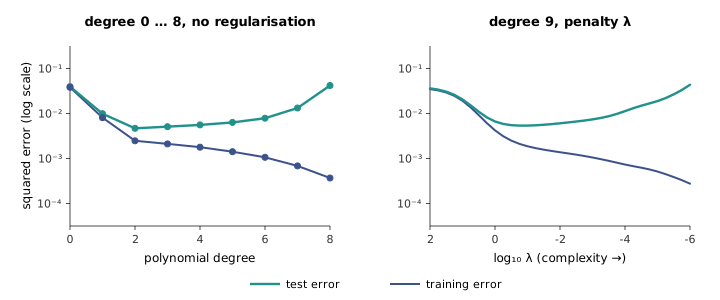
37:57 Plot error against model complexity. Training error falls monotonically: a fifth-order polynomial can always fit the training set at least as well as a fourth, because it contains the fourth as a special case. Error on new data falls at first, as the model becomes flexible enough to capture the trend, and then rises, as the extra flexibility goes into fitting noise. 39:42 The same U appears when the knob is instead of the degree, with large at the simple end. Figure 8.4 computes both curves for ten houses, averaged over 400 datasets: test error bottoms out at degree 2, at against a noise floor of , and climbs to at degree 8, while training error keeps falling.
41:32 The task is to find the bottom of the U, and it is the same task whether the knob is the degree, , the bandwidth of locally weighted regression or the of the soft-margin SVM. 42:47 The procedure is to split the data. Fit each candidate model on one part, , to get hypotheses ; measure each one’s error on the other part, ; and pick the model with the lowest dev error. “Dev” is short for development; the same set is also called the hold-out set or the cross-validation set, and Ng notes that the shorter name has won out mostly because it saves syllables. The procedure is hold-out cross-validation.
45:17 The tempting alternative, choosing the model with the lowest training error, does not work, and the left panel of Figure 8.4 shows why without further argument: the most complex model always wins on training error. Selecting on the training set would pick the fifth-order polynomial every time.
46:46 Choosing on the dev set has a cost of its own. The chosen model has now been tuned to the dev set — its parameters were fitted on and its complexity on — so its dev error is no longer an unbiased estimate of how it will do on new data. Anyone who wants to report a number, in a paper especially, needs a third set, , that played no part in any decision.
48:38 A student asks whether dev and test error usually differ by much, and Ng answers with numbers. Suppose polynomials of increasing degree score dev errors of 10, 5.1, 5.0, 4.9, 7 and 10. The winner reports 4.9; but perhaps the middle three are all really 5.0, and the one at 4.9 simply got lucky with the noise. Choosing the minimum of noisy scores systematically selects a lucky one. How lucky is computable: the expected minimum of independent standard normals is about for (the generator gets by integration and by simulation), so six models of identical true error, scored with noise of standard deviation , report on average for the winner. The bias grows with the number of models compared.
51:31 The same effect, Ng says, operates on a whole research field when everyone tunes against one public test set for years; he cites a then-recent study of CIFAR as arguing that some of the field’s apparent progress on it was overfitting to the benchmark. The study’s own conclusion is more specific (Recht et al., 2018). Its authors built a fresh CIFAR-10 test set and found that accuracy dropped by 4 to 10 percentage points across a broad range of models — but that newer models dropped less and kept their ranking, which they read as evidence against adaptive overfitting to the old test set; they attribute the drop to the models’ sensitivity to small shifts in the data distribution instead. The worry Ng describes is legitimate, but this paper is evidence for a different one.
52:29 When Ng is shipping a product rather than making a claim, he sometimes does without a test set altogether, knowing that the dev number he sees is optimistic. That is acceptable only because nobody outside the team is relying on the number. 1:00:22 The opposite case is also allowed: a team may evaluate on the test set every week and chart the result. What is not allowed is acting on it. Rolling back to last week’s model because this week’s scored lower on the test set is a decision made on the test set, and from that moment it is one more dev set.
53:33 How much data goes into each set? The historical rule of thumb is 70 % train and 30 % test, or 60/20/20 with a dev set, and Ng considers it fine for datasets of a hundred to a few thousand examples. 54:46 For very large datasets the fractions shrink: with 10 million examples, a 20 % dev set is 2 million examples, and the question is whether that many are needed. His criterion is that the dev and test sets should be large enough to detect the size of difference you care about, and no larger; the rest belongs in training. Splits of 90/5/5, or 98/1/1, are common at that scale.
55:40 His example is online advertising, where a team might ship ten projects that each raise the click-through rate by 0.01 %. To tell 90 % from 90.01 % accuracy, he says, a hundred examples cannot do it, and you need “at least 1,000 examples and maybe 10,000 or more”. That last figure is the size at which a single example is worth 0.01 % — the resolution of the measurement — but resolution is not detectability. The standard error of an accuracy near 90 % measured on examples is :
| Dev-set size | One example is worth | Standard error of a 90 % accuracy |
|---|---|---|
| 100 | 1 % | 3.0 % |
| 1,000 | 0.1 % | 0.95 % |
| 10,000 | 0.01 % | 0.30 % |
| 1,000,000 | 0.0001 % | 0.03 % |
At 10,000 examples the noise is thirty times the difference being sought. Two independently measured accuracies 0.01 % apart are only two standard errors apart at around million examples. Comparing both classifiers on the same examples helps a great deal, because the noise then comes only from the examples on which they disagree; but even then a 0.01 % difference needs tens of thousands of examples at the very least. Ng’s broader point stands and is, if anything, understated: small improvements need very large evaluation sets. The same table shows that his other example, telling apart algorithms 1 % apart with 1,000 examples, is about one standard error — enough for a hint, not for a verdict.
8.5 k-fold and leave-one-out cross-validation
1:02:10 Hold-out validation is wasteful when data are scarce. Ng’s group has worked on medical datasets in which every example is a patient, collected, as he puts it, through “a lot of literal pain”. With 100 examples, a 70/30 split trains every candidate on only 70 of them and then judges it on only 30, which is a noisy judge.
1:04:09 k-fold cross-validation recycles the data. Split into disjoint pieces of examples each. For each candidate model, and for each , train on all the pieces except and measure the error on ; the model’s score is the average of those errors. Pick the model with the best score. Ng draws to keep the board legible, but is by far the most common choice. 1:13:51 The averaging is of the held-out errors, which are just numbers — a squared error of 5.0 on one fold, 5.7 on the next, 2.8 on the next — not of the models.
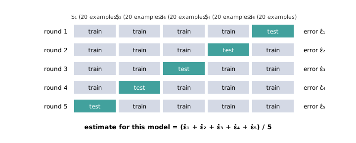
1:07:41 At the end there are trained copies of the winning model, each fitted on of the data. One could keep all of them and average their predictions, but the more common final step is to refit the chosen model once on all of . With each round holds out 10 % of the data rather than 30 %, so the models being compared are trained on nearly as much data as the final one; the price is fitting every candidate ten times.
1:09:31 Taking gives leave-one-out cross-validation: train on all but one example, test on that one, and repeat for every example. It is the most data-efficient version and the most expensive, fits per model. Ng uses it only when is roughly 100 or less, and would switch to k-fold somewhere between 20 and 50 examples. For linear models with a squared-error loss the expense is an illusion, because the leave-one-out residuals can be read off a single fit: if is the matrix that maps the targets to the fitted values ( is the identity with a zero for the intercept), then the error on example when it is held out is . The generator computes leave-one-out error both ways, by refits and by this formula, and they agree to nine significant figures; it is how the of Figure 8.3 was chosen.
1:11:38 A student asks whether the spread of the ten fold errors gives a variance for the cross-validation estimate. It does not, quite, because the ten errors are correlated: any two of the ten training sets share eight-ninths of their examples. Ng recalls research by Michael Kearns on how correlated they are and says the theory does not settle it. The cleaner result came later: Bengio and Grandvalet (2004) proved that no unbiased estimator of the variance of k-fold cross-validation exists. The naive estimate errs low. On forty houses with a quadratic and , the actual variance of the cross-validation estimate across 1,500 datasets is 1.21 times the average of what the folds’ own spread suggests.
1:12:46 Cross-validation is rare in deep learning, Ng adds, because training a network ten times is expensive, and with only twenty examples a network needs other help anyway, such as transfer learning. 1:15:32 And how should examples be assigned to the sets? Shuffle at random, provided all the data come from one distribution. When training and deployment data differ, as when speech recorded on phones is used to build a smart speaker, splitting becomes more delicate; Ng defers that case to his book Machine Learning Yearning and to CS230.
8.6 Feature selection
1:17:00 Feature selection is model selection where the models are subsets of features. It makes sense when there are many features and one suspects only a few matter: of 10,000 word indicators, stop words such as “the” and “of” say nothing about whether an email is spam; of the hundreds of sensor readings on a truck, perhaps a handful predict a breakdown. It does not make sense for images, where every pixel carries a little information. Ng stresses that deciding which regime one is in takes judgement.
With features there are subsets, far too many to try, so the search is greedy. 1:19:09 Forward search starts from the empty set — the model , which predicts the average — and repeats one step: for every feature not yet in , fit the model on plus that feature and evaluate it on the dev set (or by cross-validation); then add the feature whose addition helped most. 1:20:18 With five features, the first round fits five one-feature models; if wins, the second round fits four models of the form ; and so on, stopping when adding a feature no longer helps, or running to the end and returning the best subset seen. Backward search runs the other way, starting from all features and removing one at a time.
The generator runs forward search on five features of which only and matter. It adds , then , and after that dev error stops moving (0.320, 0.319, 0.322, 0.328 as the three irrelevant features are added). Run to the end, forward search makes fits — 16 for five features, the count the generator verifies — which is quadratic rather than exponential in . That is the sense in which it is affordable, and also the sense in which Ng calls it expensive: for 10,000 features it is fifty million fits.
cs229-notes5, section 2, also covers filter feature selection, which scores each feature on its own — for instance by its mutual information with — and keeps the top , choosing by cross-validation. It is much cheaper than forward search and is the usual choice for naive Bayes on text.