13 Expectation-Maximization Algorithms
Lecture 13
k-means clustering, anomaly detection, mixture of Gaussians, EM algorithm, Jensen’s inequality
Lecture video: Lecture 13: Expectation-Maximization Algorithms · 1:20:31
Based on the lecture by Andrew Ng — CS229, Stanford University, Autumn 2018.
In unsupervised learning the training set is with no labels, and the job is to find structure in it. This lecture builds two algorithms that alternate between a guess about hidden structure and a fit given that guess. k-means guesses which cluster each point belongs to and moves each cluster’s centre to the mean of its points. The EM algorithm for a mixture of Gaussians does the same with probabilities instead of hard assignments. The second half derives EM in general. Each E-step builds a lower bound on the log-likelihood that touches it at the current parameters, and each M-step maximises that bound, so the likelihood can never decrease. Jensen’s inequality is the tool that makes the bound.
The same derivation carries the next lecture’s factor analysis, which is why Ng gives it in full rather than stopping at the intuitive version.
13.1 k-means
2:19 Ng opens with an animation (Figure 13.1). Given unlabelled points that seem to form two groups, place two cluster centroids at random. Then repeat two steps: colour every point by the centroid it is closer to, and move each centroid to the mean of the points of its colour. After a few rounds the colours stop changing and the centroids stop moving, and the algorithm has converged.
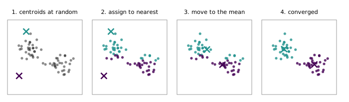
5:42 Written out, the algorithm is:
- Initialise the cluster centroids .
- Repeat until convergence:
- for every , set ;
- for every , set .
The first inner step assigns each example to its nearest centroid. The second moves each centroid to the average of the examples assigned to it. 6:23 The animation drops the initial centroids at arbitrary positions, but Ng points out that the usual practice is to set them to training examples chosen at random. In two dimensions this hardly matters, but in high dimensions a random vector tends to land far from all the data and capture no points.
The most common use Ng names is market segmentation: group a website’s users into types that can be targeted differently, without anyone having labelled what the types are. The Google News clustering of stories from the first lecture is another.
13.2 The cost k-means descends
11:45 k-means is guaranteed to converge, and the proof is a cost function. Define the distortion
the total squared distance from each point to the centroid it is assigned to. The assignment step minimises over with fixed, since each term is minimised separately by choosing the nearest centroid. The update step minimises over with fixed, because the point that minimises a sum of squared distances to a set of points is their mean. So k-means is coordinate descent on , and never increases. Since it is bounded below by zero, it must converge. The generator tracks after every half-step of every run and confirms it never rises. In Figure 13.1 it falls from 476.9 to 31.3 in three rounds. On very large data sets, Ng adds, people often stop once the decrease in has become small, without waiting for convergence.
8:49 A student asks whether the norm in the circulated notes is an norm. Ng says it is , the default whenever a norm is written without a subscript, and adds that with or without the square “the algorithm is the same either way”. For the assignment step that is right. Squaring is monotone on non-negative numbers, so the nearest centroid is the same under and , and the generator confirms identical assignments for 200 random sets of centroids. For the update step it is not. The mean minimises the sum of squared distances. The point that minimises the sum of plain distances is a different one, the geometric median, so the convergence argument above only works for the squared cost. The generator finds random starts where moving to the means raises the unsquared cost: 26 of 2,000. So k-means does descend a cost, but it is the squared one, Equation 13.1.
13:33 Ng is most often asked how to choose . He usually chooses it by hand, for two reasons. Unsupervised data is often genuinely ambiguous: the same picture can look like two clusters to one person and four to another. And criteria that pick automatically, such as AIC and BIC, answer a question the application did not ask. The better guide is what the clusters are for. If the marketing team can run four campaigns but not a hundred, use four clusters. In image compression, choose by how much compression you want.
15:41 k-means can stop at a local minimum of , since coordinate descent only guarantees that stops decreasing. The fix Ng gives is to run it many times from different random initialisations and keep the run with the lowest . On three well-separated clusters, the generator’s 100 restarts, each initialised at three random training examples, ended at seven different final costs, from 92.6 to 378.2, and the best was reached 92 times. Taking the lowest cost over a handful of restarts is therefore cheap insurance.
13.3 Density estimation and anomalies
16:18 A related but different problem is density estimation: model from unlabelled data. Ng’s example comes from friends who worked on aircraft engines. As each engine comes off the assembly line, measure its vibration and the heat it produces. If a new engine’s measurements fall where is very small, flag it and send it for inspection before it is fitted to a plane. The same scheme finds cell towers whose network traffic has turned strange, and computers sending unusual traffic.
19:46 The interesting anomaly in his sketch is one where neither feature is unusual on its own. Many engines vibrate that much, and many run that hot, but few do both. Only a joint model of catches it. And the data he draws are L-shaped, which no single textbook distribution fits. They look instead like two Gaussian blobs, perhaps engines from two production processes, which is the idea of the next section.
13.4 The mixture of Gaussians
24:23 The model introduces a latent random variable , meaning one that exists but is never observed. For each example,
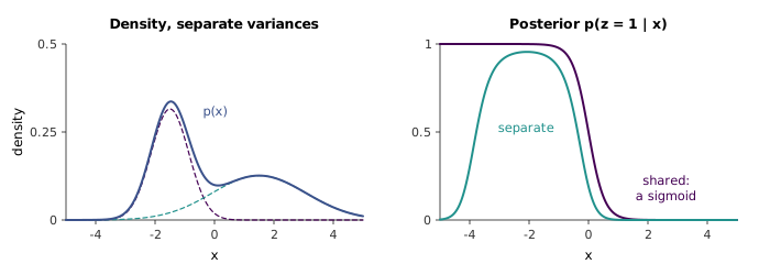
where , , . In words: pick one of Gaussians with probabilities , then draw from it. The density of is the mixture , which with enough components can take almost any shape, such as an L, or a narrow peak beside a wide hump (Figure 13.2, left).
This is Gaussian discriminant analysis (Section 5.3) with two cosmetic differences: takes values instead of two, and each component has its own covariance by convention, where GDA shared one. The real difference is that GDA’s labels were observed and are not. 28:12 If the were observed, maximum likelihood would give GDA’s closed-form estimates, and the mean of the examples with , and their covariance. Not knowing which Gaussian each example came from is the whole difficulty.
13.5 EM for the mixture: soft k-means
30:54 EM resolves the difficulty with the same bootstrap as k-means. Guess the , fit the parameters as if the guesses were labels, and repeat. The guesses are probabilities rather than hard labels.
E-step. For each and , compute the posterior probability that example came from component ,
which is Bayes’ rule, exactly as GDA used it to classify.
M-step. Re-estimate the parameters with the GDA formulas, with each indicator replaced by :
36:30 The replacement is principled: is the expected value of the indicator under the current posterior, since the expectation of an indicator is the probability of its event. 37:10 Ng’s intuition is that this is k-means with soft assignment. k-means gives each point entirely to the nearest centroid, even when it is only slightly nearer. EM gives it, say, 0.8 to one Gaussian and 0.2 to the other, and each mean becomes a weighted average in which each point counts with that strength. A student asks how to think about the weights. Ng’s reading is that each point is assigned with total strength one, split across the components. In the engine story, a point with a 10 per cent chance of coming from process one contributes a tenth of an engine to process one’s Gaussian.
The analogy can be made exact. Give all components the same fixed covariance and equal , and let . Then the posterior in Equation 13.3 goes to 1 for the nearest mean and 0 for the others, and the mean update becomes k-means’ update. In the generator’s one-dimensional example, the largest gap between EM’s soft assignments and k-means’ hard ones is once .
34:06 Ng describes the E-step for two classes as a sigmoid: the probability of the left Gaussian falls smoothly from one to zero across the gap between the means. That is GDA’s result (Section 5.4), and it holds when the components share a covariance. With equal variances the posterior is exactly , which the generator checks to . With separate covariances, the convention the model was just given, is quadratic in rather than linear, and the posterior need not be monotone. In Figure 13.2 the left component is narrow and the right one wide. The posterior of the left component rises to 0.955 near and falls back to 0.003 at , because far out on either side the wide Gaussian is the likelier source. EM handles this without any change. It only means “points on the left go to the left cluster” is not what the E-step computes.
38:56 Once fitted, the mixture gives for any new engine, and a low value flags an anomaly. Ng closes the section with a memory from a summer at AT&T Bell Labs, of a colleague who had just run EM on a mixture of three Gaussians for the first time and could not stop showing people what it did.
13.6 Jensen’s inequality
48:07 The argument so far was heuristic: guess the latent variables, then pretend they were observed. To show that EM really is maximum-likelihood estimation, Ng needs Jensen’s inequality. Let be convex, meaning , and a random variable. Then
His example takes or , each with probability one half. Then , and is the average of and , which is the midpoint of the chord joining those two points of the curve (Figure 13.3). A convex function lies below its chords, so the chord’s midpoint is above . Ng admits that he and his friends do not remember which way the inequality goes. They redraw this picture every time.
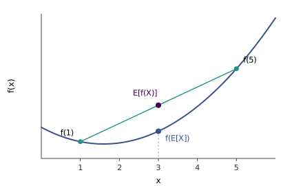
53:23 EM also needs the equality case. If is strictly convex, , then equality holds only if is constant, i.e. with probability one, which is the measure theorist’s way of saying it. A straight line is convex but not strictly, and for it equality holds for any . 54:47 A student asks about a curve with . Equal end values alone change nothing: the chord is then flat, and a strictly convex curve still dips below it in between. Equality for a non-constant needs the function to be straight between the values takes, for instance flat between 1 and 3, and such a function is not strictly convex. The strictness is the hypothesis that rules this out.
For EM the inequality is used upside down. A concave function is the negative of a convex one (), and for concave , , with equality for strictly concave only when is constant. The function it is applied to is , which is strictly concave.
13.7 EM as maximising a lower bound
57:30 Take any model with latent and all the parameters (for the mixture, ). The log-likelihood of the data marginalises out:
The sum inside the logarithm is what makes this hard. 1:19:12 A student asks at the end why we do not just maximise directly. Setting its derivatives to zero gives equations with no closed-form solution for the mixture, or for factor analysis next time, whereas each step of EM is in closed form. Gradient ascent on is possible, but it needs a learning rate, and EM needs none.
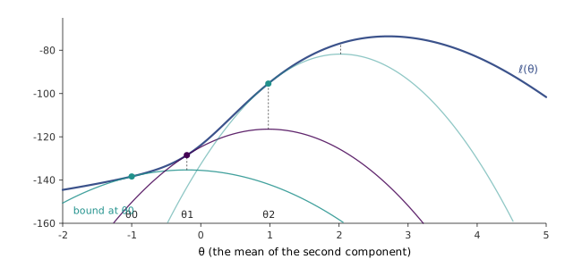
59:58 Ng gives the picture first (Figure 13.4). The E-step builds a lower bound on that has two properties: it lies below everywhere, and it equals at the current parameters . The M-step jumps to the maximum of the bound. At that point is at least as high as the bound, which is at least as high as it was at , where it equalled . Repeat, and climbs until EM reaches a local optimum. As with k-means, which local optimum it finds depends on the starting point.
1:04:21 To build the bound, pick for each example any distribution over the values of , multiply and divide by it, and read the inner sum as an expectation over :
The inequality is Jensen’s for the concave : the log of an expectation is at least the expectation of the log. The right-hand side, viewed as a function of with the fixed and the summed out, is the green curve of Ng’s picture. Today it is usually called the evidence lower bound, or ELBO.
1:11:54 The bound holds for every choice of . The E-step chooses the that make it tight at the current . By the equality case of Jensen’s inequality, that requires the random variable inside to be constant, so must not depend on . In other words, . Normalising to sum to one gives
the posterior of the latent variable given the data, which is exactly the of Equation 13.3. The general algorithm is then:
- E-step: for each , set .
- M-step: set .
For the mixture of Gaussians, the M-step’s maximisation is the weighted GDA fit of Equation 13.4, so the heuristic of the previous section was EM all along.
The generator checks each step of this argument on the one-parameter model of Figure 13.4, a mixture of and with equal weights, where only the second mean is unknown. At each of the first four iterates, the bound equals to , has the same slope (so the curves are tangent rather than merely touching), and lies below at every point of a fine grid. Its maximiser found by grid search agrees with the closed-form M-step. From the iterates run and converge to , and rises at every step, from to .
There is a caveat about “maximum likelihood” for mixtures. When each component has its own variance, the likelihood has no maximum at all. Centre one component exactly on a training point and shrink its variance. That point’s density grows without bound while the other components keep the remaining points’ densities finite, so . The generator shows rising without limit as the variance falls through , , … . EM does not usually find these degenerate solutions, because it climbs from where it starts, but a component that captures a single point can drift into one. In practice this is guarded against by restarting, or by putting a floor or a small prior under the covariances. “Converges to a local optimum” is the accurate claim, and for mixtures the global optimum is not a useful target.
k-means and its convergence as coordinate descent are in cs229-notes7a. The mixture of Gaussians and its EM updates, including the step the lecture skipped, are in cs229-notes7b. Jensen’s inequality, the general derivation, the proof that increases monotonically, and the view of EM as coordinate ascent on the lower bound are in cs229-notes8, sections 1 to 3. The original general treatment is Dempster, Laird and Rubin (1977), and the k-means iteration is Lloyd’s (1982).