18 Continuous State MDPs and Model Simulation
Lecture 18
continuous state MDPs, discretization, model-based reinforcement learning, simulator, fitted value iteration
Lecture video: Lecture 18: Continuous State MDP and Model Simulation · 1:20:15
Based on the lecture by Andrew Ng — CS229, Stanford University, Autumn 2018.
Value iteration as lecture 17 left it keeps one number per state, so it needs a state space it can list. A car, a helicopter or a pole balanced on a cart has a state made of real numbers. This lecture gives two ways to cope. The first is to chop the state space into cells and pretend it is discrete. The second is to treat the value function as something to fit: sample states, compute what value iteration says their values should be, and run linear regression on features of the state to fill in everything between. That second method, fitted value iteration, needs a simulator it can query at any state, and Ng spends the middle of the lecture on where such a simulator comes from. His preferred answer is to learn one from a pilot’s flight logs.
18.1 States that are vectors
3:43 Ng starts from three robots and asks, for each, what the state has to contain. A car seen from above needs its position and its heading . That is enough at walking pace, but at any real speed the next position depends on how fast the car is moving, so the state also carries the velocities : six numbers. Whether to add the steering-wheel angle or the wear on the tyres is a modelling choice that depends on what you are building. A helicopter moves in three dimensions, so it has position , an orientation given by roll, pitch and yaw , and the six corresponding velocities: twelve numbers. The third robot is the classic toy of early reinforcement learning, the inverted pendulum: a cart on a rail with a pole hinged freely on top, which the controller must keep upright by pushing the cart left and right. Its state is , four numbers.
10:06 In all three, with equal to 4, 6 or 12. Angles wrap around rather than run along the real line, which a mathematician would object to; for the algorithms in this lecture the distinction does not matter.
18.2 Discretization, and what it costs
10:55 The direct approach lays a grid over the state space, gives every cell a name, and treats the robot as being “in” a cell whenever its true state falls inside it. The continuous problem becomes a discrete MDP that value iteration can solve, and the policy for a continuous state is the policy of its cell. Ng is clear that this is often fine. For a low-dimensional problem it is the quickest thing to get working.
12:31 It has two weaknesses, and he makes the first one with the example the course opened with. Suppose you predicted house prices by cutting the size axis into five intervals and fitting a constant on each. You would get a staircase, a poor representation of a price that varies smoothly with size. Discretizing the state space does exactly this to the value function: is approximated by a constant on every cell. The left of Figure 18.1 shows the staircase on a one-dimensional MDP of our own. The state is a point on a line, the actions move it left, right or not at all by 0.25 with Gaussian slip of standard deviation 0.15, the reward is , and . With six cells, the discretized value function misses the true by up to 14.8. Doubling the cells halves the error, to 7.0, then 3.4 and 1.8 with 48 cells. The dashed curve is the method the rest of the lecture builds, which fits five numbers and lands within 1.8.
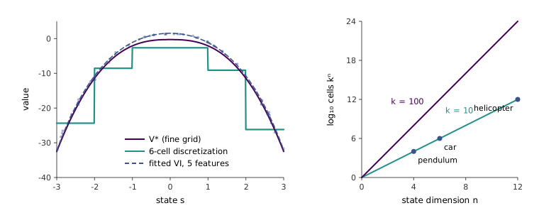
14:35 The second weakness is the one Bellman named the curse of dimensionality. Discretizing each of state variables into values gives cells. At a coarse the pendulum needs cells and the car . The helicopter needs , and the official notes’ example of a 10-dimensional state at 100 values each needs (right of Figure 18.1). Ng adds that the curse is not only about continuous states. A factory with 100 machines, each in one of conditions, has discrete states, and fitted value iteration can be the better algorithm there too.
17:25 His working rules for when to discretize are worth having as stated. In two or three dimensions, just do it. In four to six, think about it, and it will often still work. The pendulum is fine, and friends of his made a six-dimensional bicycle model work “if you put some work into it”. The usual trick in this range is to discretize unevenly, spending more values on the variables the policy is most sensitive to, because every value saved is saved in the exponent. At seven or eight dimensions he becomes nervous. Above that he would very seriously look for an algorithm that does not discretize. The official notes draw the line a little lower: they promise reliable results in one or two dimensions, four with care, and six only with luck.
18.3 Getting a model
23:20 Fitted value iteration needs a model, or simulator: a black box that takes a state and an action and returns a next state drawn from . For simplicity the action space is taken to be discrete. Ng points out that this is usually a mild assumption, because robots tend to have far fewer controls than state variables. The car has a six-dimensional state but two controls, steering and braking. The helicopter has twelve state variables and four controls, a stick under each hand that moves in two directions. The pendulum has four and one.
26:13 One way to get a simulator is physics. For the pendulum, Newtonian mechanics gives as a function of the state, the push and the masses and length of the parts. Ng shows the equation only as decoration. Stepping it forward as with s simulates the system at 10 Hz. In practice nobody derives these by hand. You download an open-source physics engine and give it the dimensions. He once built a four-legged walking robot’s controller this way.
29:15 The way he uses more often is to learn the model from data. Take the helicopter into a field and have a human pilot fly it around while GPS, accelerometers and a compass log the state ten times a second, along with the stick positions. One flight gives a trajectory ; repeat it times. Predicting from is now a supervised learning problem. Its linear version is
with square and tall and thin when the action has components. Ng’s verdict from experience is that this is “actually not a terrible model” for a helicopter flying slowly and roughly level, and a poor one for fast, aggressive manoeuvres. Nonlinear features and can replace the raw state and action when the linear model is not enough.
Equation 18.1 looks like a new kind of regression because and are matrices. Ng’s remark that it is the same as running ordinary linear regression times, once per state variable, is right: the squared norm is a sum over the components, and each component involves only one row of . The notes add that the least-squares fit is also the maximum-likelihood one. That holds even if the noise in different state variables is correlated, which is the realistic case, because every equation shares the same regressors. The generator confirms all three routes on a simulated two-dimensional system with correlated noise. The joint fit, the separate regressions and the Gaussian maximum-likelihood fit with the true covariance agree to .
35:37 A student asks whether short flights differ from one long one. For the algorithm, Ng says, they do not. In practice the helicopter burns fuel and gets lighter, and the wind changes, so several flights average over conditions a single one would not cover.
37:41 Having fitted and , there are two simulators to choose from. The deterministic one sets . The stochastic one adds , whose covariance can be estimated from the residuals, and draws a fresh on every step. This whole approach of learning a model and then planning in it is model-based reinforcement learning. The alternative, model-free RL, runs the learning algorithm on the real system directly. Ng’s view in 2018 is that model-based methods were taking off faster in robotics. A physical robot cannot afford to be crashed thousands of times while it learns, while a video game or a board game is its own perfect simulator and can be.
41:45 He ends this part with a lesson from many robots. A policy optimised against a deterministic simulator tends to be brittle. It exploits details of the simulator that the real machine does not share, and that is how a five-legged robot can walk beautifully in a video and fall over in the lab. A simulator is always a little wrong: it misses a wind gust, or banks a degree too far in a turn. If the policy has to work in a slightly noisy simulator, it is much more likely to work on the real robot. His advice is to always add noise. The exact distribution matters much less than remembering to add it. (He mentions in passing that his own PhD thesis used reinforcement learning to fly helicopters, and that he lived through the crashes.)
18.4 Fitted value iteration
46:13 With a simulator in hand, the value function is approximated the way a price is approximated in linear regression:
where is a vector of features of the state chosen by hand. Ng’s advice on choosing them is to remember what a value is: the expected payoff from that state, so features should say how well the robot is doing. For the pendulum, a pole leaning far to the right is bad unless the cart is moving fast to the right to catch it. So the product of the pole angle and the cart velocity is a natural feature, alongside , and squares. A model-based method also makes overfitting less of a worry than in ordinary supervised learning. The training data come from the simulator and cost nothing, so a generous set of features, some of which turn out useless, can be fitted from as many samples as the computer can afford.
50:14 The algorithm starts from value iteration’s update in continuous form,
and replaces the two things it cannot do. It cannot visit every state, so it visits a sample. It cannot store an arbitrary , so it fits Equation 18.2 to the targets that Equation 18.3 produces at the sampled states:
- Sample states at random, and set .
- Repeat:
- For each and each action : draw from the simulator and set .
- Set .
- Set .
56:46 Each is a sample-average estimate of the expectation in Equation 18.3, so is an estimate of the whole right-hand side at . 58:04 Discrete value iteration would now set , but a linear function cannot have its values set one point at a time. The best it can do is come as close as possible to all the targets at once, which is a least-squares fit. Step (c) is linear regression with in the role of and in the role of the price. A student asks where in step (a) comes from. 1:08:35 It is with the from the previous iteration, exactly as discrete value iteration uses the previous sweep’s values.
1:00:51 Two questions clarify the bookkeeping. The here is the number of sampled states and has nothing to do with the flights used to learn the model. Ng’s picture is one team flying the helicopter a thousand times and publishing a model, and another team running fitted value iteration on it. 1:03:06 He then asks the class how the algorithm simplifies with a deterministic simulator. The answer is that suffices, since all samples would be the same next state. The generator checks this mechanically: with the noise switched off, and give the same to within . On how large should be, 1:05:38 he reasons as for any regression. With 50 features, 500 samples might do. But samples are free, so there is no harm in 5,000 or 100,000 beyond running time. 1:09:07 Finally, nothing requires the regression to be linear. Locally weighted regression works, and replacing it with a neural network is, he says only half joking, how you get deep reinforcement learning.
On the one-dimensional MDP of Figure 18.1, with 200 sampled states, and five polynomial features, fitted value iteration lands within 1.8 of everywhere. That is as good as the 48-cell discretization, using five numbers instead of 48. With only three features, , the error is 7.1. The true is not exactly quadratic, and a fit can only be as good as its features.
What the lecture does not say, and the notes do in one sentence, is that fitted value iteration “cannot be proved to always converge”. Discrete value iteration converges because its update is a contraction in the max norm (Section 17.3). A least-squares fit is not a max-norm operation, and composing the two can expand distances instead of shrinking them. Tsitsiklis and Van Roy give the smallest example, reproduced in Figure 18.2. There are two states with no actions and no rewards; state 1 moves to state 2, which stays put, so . There is one feature, in state 1 and in state 2. The targets are for both states, and the least-squares fit of to them is
so grows geometrically whenever . This happens although the features represent exactly at . The cause is that the fit weights both states equally while the dynamics send everything to state 2. The algorithm as written starts at , and in this example it would sit there for ever. Any nonzero start, or any noise in the targets, sets the divergence going.
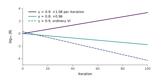
None of this makes the algorithm unusable. The notes say it usually converges or nearly converges in practice. At the start of lecture 19 Ng answers a student who asked whether it really works: it does, on a real helicopter at low speed. The counterexample is a reason to watch across iterations rather than trust it.
Discretization, simulators, learning a linear model and fitted value iteration are in cs229-notes12, section 4, which also writes the update with an integral over and states the convergence caveat.
18.5 From a value function to an action
1:10:37 Fitted value iteration returns , and is only implicit in it:
On a helicopter this has to be computed ten times a second. The obvious method is to estimate the expectation from simulator samples, as in training. Ng is reluctant to do that. He does not like the idea of a self-driving car with a random number generator in its control loop, where an unlucky draw could pick a bad action. 1:13:35 The common fix uses the form most simulators have, . Train with the noise, so that the policy is robust, but at deployment set and :
Each tenth of a second the controller simulates one step for every action, evaluates at the predicted next states, and takes the best. Ng admits this is not rigorously justified. There is one case where it is exact. If is quadratic and the noise is additive with a distribution that does not depend on the action, then
for zero-mean noise with covariance , where is the (constant) Hessian of . The second term is the same for every action, so dropping the noise cannot change the argmax. The generator confirms that the quadratic fit’s two read-outs agree at every one of 601 states. For other features the noise term depends on , so the two can disagree, though in this toy the quartic fit still never did. This is a first glimpse of a fact lecture 19 makes central: for quadratic values and linear-Gaussian dynamics, the noise does not change the optimal action at all.
1:18:26 Asked about continuous actions, Ng says a car’s steering and braking can be discretized without much loss, but a helicopter’s controls usually are not. When is smooth, the maximisation in Equation 18.4 can be done by a fast numerical optimiser in real time, which is the territory of model predictive control. 1:19:24 And to a student asking how the controller knows where it has got to after acting: it measures. A tenth of a second later a new GPS reading and new sensors give the new state, wind and model errors included, and the argmax is taken again from there.