9 Decision Trees and Ensemble Methods
Lecture 9
decision trees, cross-entropy loss, bagging, random forests, boosting, AdaBoost
Lecture video: Lecture 9: Decision Trees and Ensemble Methods · 1:20:41
Based on the lecture by Raphael Townshend, head TA — CS229, Stanford University, Autumn 2018.
A decision tree splits the input space into rectangles by asking one yes-or-no question about one feature at a time, and predicts a constant in each rectangle. It is the course’s first genuinely non-linear model, it is easy to explain to anyone, and on its own it is not very accurate: a fully grown tree has low bias and very high variance. The second half of the lecture is about the cure, which is to average many trees. Averaging cuts variance by an amount the correlation between the trees controls, and that single formula explains bagging, the extra randomness of random forests, and why boosting, which works on bias instead, uses deliberately weak trees.
The lecture is given by Raphael Townshend, one of the course’s head TAs, while Ng is travelling. It is almost entirely board work, built on one running example.
9.1 A model that cuts the space into boxes
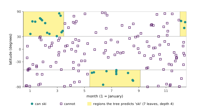
1:24 Townshend, who is Canadian and likes to ski, poses a classifier: given a month and a latitude, can you ski there? Plot month (1 for January to 12 for December) against latitude ( at the North Pole, at the South). The positives sit in two separate blocks, the northern winter at high northern latitudes and the southern winter, mid-year, at high southern ones, with nothing near the equator. No line separates that, and while a kernel might lift it into a space where a hyperplane does, the structure is plainly a set of boxes, and it would be simpler to find the boxes directly.
3:38 Finding the best set of regions is intractable in general. A decision tree finds a good one greedily, top-down and recursively. It starts with the whole space and asks the single question that best separates the classes — “is the latitude above 30°?” — which cuts the plane in two. It then treats each half as a fresh problem and asks another question there, “is the month before March?”, and so on: a game of twenty questions with the data. Figure 9.1 shows the result on synthetic ski data. Seven leaves isolate both skiing seasons.
6:08 Formally, a split of a parent region is a feature and a threshold , which divide it into two children:
Each leaf predicts the most common class among the training examples that land in it. What remains is to say which is “best”.
9.2 Choosing a split
8:32 Define a loss for a region and choose the split that reduces it the most, from the loss of the parent to the combined loss of the children. Since the parent’s loss is fixed, this is the same as minimising the children’s loss. With the proportion of the region’s examples in class , the obvious loss is the misclassification rate, : predict the majority class and count everything else as an error.
12:29 Townshend’s example shows why that loss is the wrong one. A region holds 900 positives and 100 negatives. One split sends 700 positives and 100 negatives one way and 200 positives the other; another sends 400 and 100 one way and 500 positives the other. The second split looks better — it isolates a pure region of 500 — but both children of both splits still predict “positive”, so each split makes exactly the 100 mistakes the parent made. Misclassification registers no gain for either, and a tree built on it would have no reason to prefer the split that obviously helps.
15:21 The fix is a loss that rewards purity even when it does not change any prediction. The standard choice is the cross-entropy,
the number of bits needed, on average, to tell someone the class of an example when they already know the proportions: zero for a pure region, one bit for a 50/50 binary region. 51:56 Asked whether the logarithm must be base 2, Townshend is “pretty sure” it does not matter. It does not: changing the base multiplies every loss and every gain by the same constant, so the ranking of splits cannot change. The generator confirms the ratio is exactly for both splits.
One detail on the board needs care. The children’s loss must be weighted by their sizes,
as cs229-notes-dt writes it. The board writes , which is correct for misclassification measured in counts, as in the example, but not for losses defined on proportions such as Equation 9.1. Unweighted, the sum can be made larger than the parent’s loss by peeling off a single positive and a single negative — a region of two with a full bit of entropy — even though such a split barely changes anything. With the weighting, cross-entropy gives the lecture’s two splits gains of and bits, preferring the second as intuition does.
21:44 The geometry explains why this works, and Figure 9.2 draws it. Plot a binary loss against , the share of positives. A parent’s is the size-weighted average of its children’s, so the parent sits on the curve at that average, while the children’s weighted loss sits on the chord between the children’s points. For a strictly concave curve such as cross-entropy, the chord lies strictly below the curve whenever the children differ, so every split that changes the class proportions gains something. Misclassification is a tent, linear on each side of . When both children fall on the same side as the parent, the chord lies on the curve and the gain is exactly zero, which is what happened in the example. Over random splits of random regions the generator finds this case — positive cross-entropy gain, zero misclassification gain — in about half of all splits.
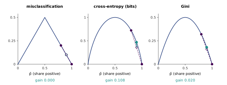
29:36 The Gini impurity has the same shape and is the other common choice. It is tempting to treat the two as interchangeable, and usually they are; but the generator, offering both the same ten random candidate splits of a 60/40 region 2,000 times, finds that they choose different splits in of cases. The family resemblance is the concavity, and that, Townshend says, is what the losses that work in practice have in common.
9.3 Regression trees and categorical features
31:03 Nothing above depends on the labels being classes. To predict snowfall instead of “can ski”, let each leaf predict the mean of its targets, , and measure the region by squared error, . These are regression trees, and splitting proceeds exactly as before. 34:34 Asked how the best split is actually found, Townshend says it is found by brute force, efficiently: sort the examples along each feature, and every distinct gap between consecutive values is a candidate threshold that can be scored with running sums in one pass.
35:06 Trees also take categorical features naturally. If location is one of north, equator or south, a split is a question such as “is the location in the northern hemisphere?” — in general, “is the category in subset ?”. 36:27 The catch is the number of subsets. The lecture counts for categories; the number of distinct binary splits is , since a subset and its complement define the same split and the empty set defines none. Either way it is exponential. 37:01 For binary classification there is a well-known escape, which the lecture mentions without proof: sort the categories by their proportion of positives, and the best split is always one of the splits of that sorted list into a prefix and a suffix. The generator checks this against brute force over all subsets for 500 random six-category problems under cross-entropy, and the two always agree.
cs229-notes-dt, sections 2 to 4.1, give the recursive partitioning algorithm, the size-weighted split criterion and the treatment of categorical variables.
9.4 Regularising a tree
37:39 Grown until every leaf is pure, a tree can put each training example in a region of its own. That overfits, and trees are in this sense high-variance models. 38:24 The usual controls are heuristics: stop splitting a node with fewer than a minimum number of examples, cap the depth, or cap the number of nodes.
39:07 A fourth heuristic, stopping when the best split decreases the loss by less than some threshold, is one Townshend calls “very tempting” and advises against. Interactions between features can make the first question worthless on its own and the second one decisive. In the ski data the latitude question alone helps little; the latitude question followed by the month question nails it. The extreme case is XOR: label a point positive when exactly one of its two coordinates exceeds a threshold. The generator builds a balanced XOR set of 64 points, on which every single split leaves the cross-entropy exactly where it was, so a tree that splits only on positive gain stops at the root, with 32 mistakes. Taking the zero-gain split anyway, the two children are each solved by one more split, with no mistakes at depth 2.
40:07 The better approach is to grow the tree fully and then prune it backwards: remove a split if doing so does not hurt the misclassification error on a held-out validation set — the dev set of lecture 8, used to choose the size of the tree.
9.5 Runtime
42:54 Let be the number of examples, the number of features and the depth of the tree. Prediction walks one path from root to leaf, so it costs , and for a reasonably balanced tree is about . Training is the surprise. 44:46 Each example lands in exactly one node per level, so it takes part in at most split searches, and in each it is scanned once per feature. The total is . Since is the size of the data matrix, training a tree costs about as much as reading the data times. (For continuous features the scan needs the examples sorted along each feature; the sort is done once up front, or the bound picks up a logarithmic factor.)
9.6 What trees cannot do
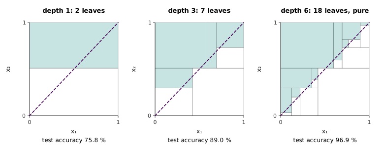
47:58 The main weakness is additive structure. Label points positive above the line . Logistic regression represents that boundary exactly with one weight per feature. A tree can only approximate it with a staircase of axis-aligned steps, and every step costs leaves. On 400 training points, a depth-1 tree reaches test accuracy, depth 3 reaches , and a tree grown until its leaves are pure stops at 18 leaves and , the staircase being as fine as the training data allow (Figure 9.3).
49:36 The scorecard, then. Trees are easy to explain — twenty questions — and short ones can be read directly. They handle categorical features and they are fast. Against that, they have high variance, they are bad at additive structure, and, mostly for those two reasons, their predictive accuracy is low. 51:09 “I know what you guys are thinking,” Townshend says: why spend half a lecture on a model that, on its own, is not very good? Because trees are the ideal raw material for ensembles, which (as of 2018) underpin many of the methods winning Kaggle competitions.
9.7 Why averaging helps
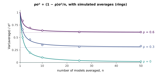
53:11 Let be independent random variables with variance . Their average has variance : each independent source divides the variance further. 55:00 Models trained on related data are not independent, though. If the are identically distributed with pairwise correlation , then
The second term vanishes as grows; the first does not. With averaging does nothing at all, and in general the variance can never fall below (Figure 9.4). 57:01 So the game has two moves: average many models to shrink the second term, and make them as decorrelated as possible to shrink the first. The generator checks Equation 9.3 by simulation for .
57:48 The most decorrelated ensembles come from different algorithms — averaging a neural network, a random forest and an SVM is a common Kaggle tactic that works well — or from different training sets, which is rarely an option, since collecting one was hard enough. Bagging approximates the second; boosting does something else.
9.8 Bagging
1:00:20 Bagging stands for bootstrap aggregation. The bootstrap is a statistician’s device for measuring the uncertainty of an estimate. The training set was sampled from a population ; ideally we would draw fresh training sets from , but we cannot. So pretend is the population, and draw new training sets from it: examples sampled from with replacement, which is what sampling from a population means. 1:03:25 Bagging takes bootstrap samples , trains a model on each, and averages:
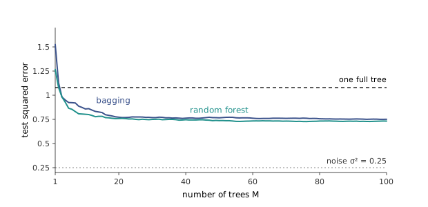
1:05:06 In the terms of Equation 9.3, the bootstrap lowers (the models see different data) and controls the second term. A consequence Townshend stresses is that more bootstrap models cannot make the ensemble overfit more: they only shrink the second term, so the usual practice is to keep adding models until the error stops falling. Figure 9.5 shows exactly that.
1:07:33 Asked how far bootstrapping can push down, he has no formula, only the reason there is a floor: every bootstrap sample is drawn from the same , and each contains about two-thirds of it. The exact fraction of distinct examples is , which the generator confirms by sampling. 1:08:29 That missing third is also the price: each model trains on fewer distinct examples, so bagging slightly raises bias. In Figure 9.5 a single tree on a bootstrap sample has test error against for one tree on the full data, but by three or four trees the average has overtaken the full-data tree, and a hundred bagged trees reach .
1:11:23 This is why trees and bagging belong together. A deep tree has low bias and high variance; bagging trades a little bias for a large cut in variance; and so a model whose error is mostly variance gains the most. Bagging a high-bias model would gain little.
The method is due to Breiman (1996).
9.9 Random forests
1:12:29 A random forest is bagged trees with one more source of randomness: at each split, the tree may only consider a random subset of the features. 1:13:56 Townshend gives two reasons this helps, which are the same reason. It lowers . And concretely, if one feature is a very strong predictor, every bagged tree will split on it first whatever its bootstrap sample, so the trees are alike from the root down; forbidding it at some splits forces them apart.
The decorrelation is real and easy to measure. On the problem of Figure 9.5 — eight noisy measurements, five of one latent variable and three of another — the correlation between two bagged trees’ predictions across training sets is about ; letting each split see only three features drops it to , with each tree’s own variance roughly unchanged, so falls from about to . The test error of 100 trees falls from with all features to about with two to four.
But the argument above is only about variance, and the lecture does not mention the other side. Forbidding a feature can also make a tree worse. On a second problem where one feature carries most of the signal and the others are weak, restricting each split to two of six features roughly doubles each tree’s variance — many splits must make do with weak features — and the forest’s test error rises from to ; with one feature per split it reaches . Random feature selection pays when the features it forces the trees to use are nearly as good as the ones it hides, as with redundant or correlated measurements. The number of features per split is a hyperparameter to tune like any other, which is how Breiman (2001) treated it.
9.10 Boosting
1:15:16 Bagging fights variance. Boosting works in the opposite direction: it reduces bias, by building an ensemble additively, each new model trained to fix what the previous ones got wrong. It starts from deliberately weak models — typically decision stumps, trees of depth one that ask a single question. A stump has high bias and low variance, which is the right raw material for a method that lowers bias. (The lecture’s sentence at 1:16:44 runs these two the wrong way round, saying that restricting to depth one decreases bias before saying it increases it; the second is right.)
1:16:59 The first stump draws its line and misclassifies some examples. Boosting increases the weight of those examples and trains the next stump on the reweighted set, which pushes it to get the hard ones right; and so on, each example’s weight reflecting how often the ensemble so far has got it wrong. Figure 9.6 runs it on the diagonal boundary that defeats a single tree. 1:18:17 Each stump also gets a vote , larger for more accurate stumps, and the final classifier is the weighted vote . The algorithm is AdaBoost, due to Freund and Schapire (1997). In the form the official notes give, with labels and weights starting at , each round:
- fits a stump to the weighted data;
- computes its weighted error ;
- sets its vote to the log-odds ;
- multiplies the weight of every misclassified example by .
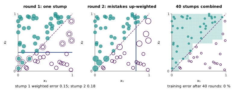
The weights look arbitrary, and the notes justify them: AdaBoost is forward stagewise additive modelling under the exponential loss , adding one stump at a time and choosing each stump’s coefficient to minimise that loss with the earlier ones fixed. That derivation gives a coefficient of — half the vote above. The generator runs both versions side by side for 40 rounds: they choose the same stump every round, their coefficients differ by a factor of exactly 2, and since doubling every vote does not change the sign of the sum, they make the same prediction everywhere on a fine grid.
On the diagonal data the first stump has weighted error and the second . Training error is after two rounds, after five, after ten, and zero from round twenty, each stump being only a little better than chance — by round 40 the newest stump’s weighted error is . Freund and Schapire’s bound guarantees this kind of progress: training error is at most , which shrinks geometrically as long as every stump beats chance by some margin. The generator asserts the bound at every round; it is at round 20 and at round 40.
The additive structure that trees lack (Section 9.6) is exactly what boosting adds, since the ensemble is a sum. That cuts both ways, and the notes say so where the lecture does not: because each new model depends on the earlier ones, adding rounds raises the risk of overfitting, unlike adding trees to a bagged ensemble. The number of rounds is chosen on held-out data. 1:20:08 The same stagewise idea with other losses gives gradient boosting, and with engineering on top, XGBoost.
cs229-notes-ensemble, section 1, covers the bootstrap, aggregation and their combination with trees; section 2 gives AdaBoost, states that it is forward stagewise additive modelling under the exponential loss (leaving the derivation to The Elements of Statistical Learning, section 10.4), and sketches gradient boosting.