10 Introduction to Neural Networks
Lecture 10
neural networks, logistic regression, softmax, forward propagation, vectorization
Lecture video: Lecture 10: Introduction to Neural Networks · 1:20:14
Based on the lecture by Kian Katanforoosh — CS229, Stanford University, Autumn 2018.
A neural network is logistic regression repeated and stacked. One neuron computes a linear function of its inputs and passes the result through a non-linearity; a layer is several neurons reading the same inputs; a network is layers feeding one another. This lecture builds that up one step at a time from a classifier the course already has, and at each step asks the same three questions: what the output means, what the loss must therefore be, and how many parameters there are. It ends with the forward pass written in matrices, for one example and for a whole batch, and with the reason gradients are computed from the last layer backwards, which the next chapter works out in full.
The two deep-learning lectures are given by Kian Katanforoosh, who teaches CS230, the Stanford deep-learning course. 1:02 He opens with the usual account of why the methods took off when they did: GPUs made the computation affordable, the digitised world made large datasets available, and these models are flexible enough to keep improving as the data grows, which older methods mostly stop doing.
10.1 Logistic regression as one neuron
3:05 The running task is to say whether an image contains a cat: output a number close to 1 if it does and close to 0 if it does not. A colour image of pixels is three such grids, one per red, green and blue channel, so it is numbers. Logistic regression needs a vector, so the first step is simply to flatten the image into a column vector , and then
This is the model of Section 3.6 with the intercept split out: with a constant feature becomes , where plays the role of and holds the rest. 6:03 Since is a scalar and is , must be a row vector, . The lecture asks for that shape before anything else, and the habit of checking shapes first carries the whole of the next chapter.
Training is the familiar loop: initialise and , minimise the logistic loss
by gradient descent, then predict with the fitted parameters. The loss is the negative log-likelihood of the Bernoulli model, so minimising it is maximum likelihood. What Katanforoosh stresses is its role: the function we actually want, the one that recognises cats, has parameters we cannot write down, and the loss is the proxy we can optimise in their place.
10:26 The model has weights and one bias. There is a quicker way to count that the lecture uses from here on: draw the model with one edge from each input to the neuron, and there is one weight per edge and one bias per neuron. It also shows something unwelcome, that the parameter count grows with the size of the input. A larger image means a larger , and the lecture flags this as something to change later; convolutional networks, which share weights across the image, are the change.
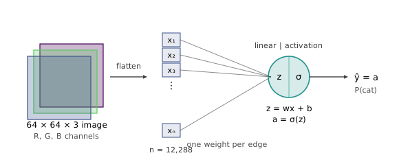
11:34 Two slogans come out of this. The first is that a neuron is a linear part plus an activation: , then , with the sigmoid as one choice of among several. The second is that a model is an architecture plus parameters. When a team says it has shipped a model, it has shipped two files, one describing the computation and one holding the numbers that computation uses. The rest of the lecture changes the architecture and lets the parameters, still called and , grow.
10.2 Three animals, three neurons
13:42 Now the task is to detect a cat, a lion and an iguana. The obvious extension is to put three neurons side by side, each connected to every pixel, each computing its own logistic regression:
The square-bracket superscript names the layer and the subscript the neuron within it. This network has one layer, whose neurons do not talk to one another, and its output is now a vector of three numbers. 17:08 Each neuron has its own weights, so the parameter count triples, to for .
The labels must change with the output. 18:42 An image of a cat gets , a lion , an iguana , and the loss is the sum of three logistic losses, one per entry. Which neuron ends up detecting cats is decided by nothing more than this labelling convention: the first neuron is only ever compared with the first entry, so it becomes the cat detector, and had the convention put cats second, the second neuron would have.
20:37 The same observation answers the question of an image showing a cat and a lion. Label it and nothing breaks, because the three neurons are trained independently; each sigmoid depends only on its own weights, and nothing forces the outputs to add up to anything. 22:32 As a student points out, the network is not yet a network in any interesting sense: it is three logistic regressions that happen to share an input.
23:49 The case where this design is the wrong one is when the classes exclude each other: a cell image showing exactly one of many diseases, say. The lecture’s argument is that a very rare class, the one iguana in a zoo of thousands of lions and cats, leaves its neuron almost untrained. That needs one qualification. The iguana neuron does receive a gradient on every image: the derivative of its logistic loss with respect to its logit is , which on an image without an iguana is and pushes the neuron towards saying “no iguana”. What the neuron lacks is positive examples, and a softmax does not create those either. The real reason to prefer a softmax for exclusive classes is that it builds the exclusivity into the model, which is the subject of the next section.
10.3 Softmax: one class per image
25:10 Add the constraint that each image shows exactly one of the three animals. Write the linear part of neuron as , drop the three sigmoids, and replace them by a single function of all three logits:
This is the softmax of softmax regression, derived as a generalised linear model in Section 4.7. 28:27 Its outputs are positive and sum to one, so they form a probability distribution over the classes. It can no longer say “probably a cat and probably a lion”: raising one output lowers the others. Labels are one-hot, , or , and the prediction is the class with the largest output. 30:03 The constraint also bakes in an assumption that one of the three animals is always present; if images with none of them can occur, a fourth class for “no animal” has to be added. The parameter count does not change, since the softmax has no parameters of its own: still .
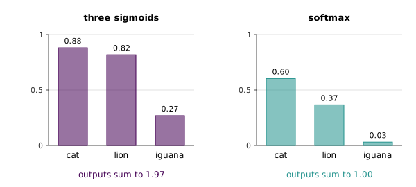
33:17 A student asks what happens if this network is trained on the multi-hot label anyway. The lecture’s guess is that it will settle near , and that is exactly right: with the cross-entropy loss below, the best a distribution can do against two targets of 1 is split its mass equally between them, and the generator, training a softmax on that label by gradient descent, ends at . The fit can never be exact, because the outputs sum to 1 and the label sums to 2.
34:07 The loss has to change too. For the three independent sigmoids the derivative of the summed loss with respect to involves only the second term, since the other two do not depend on . Under a softmax every output depends on every logit through the denominator, so the loss is the softmax cross-entropy
which for a one-hot is just of the probability given to the right class. The lecture leaves its derivative as an exercise and suggests it is harder than the sigmoid case. It looks harder and is not. The coupling through the denominator cancels, and for a one-hot label the gradient with respect to the logits is
the same form as the logistic loss of one sigmoid neuron, . The generator checks both against finite differences on 500 random logit vectors. This shared form is not a coincidence: both are canonical-link GLMs (Section 4.4), and it is the reason the next chapter’s backpropagation starts from “prediction minus label” at the output whichever of the two is used.
10.4 Predicting a number
37:17 Suppose instead the network has to estimate the cat’s age. One answer, from the room, is to treat each age as a class and use a softmax, since a cat has exactly one age. The other is to make it a regression, and that changes two things. The sigmoid at the output has to go, since it confines to . With the identity in its place, the one-neuron model is linear regression. 39:29 A better choice here is the rectified linear unit,
which is linear for positive inputs and zero for negative ones, a natural fit for a quantity that cannot be negative. The loss changes as well, to the absolute or squared error between and . The lecture’s reason is that these are easier to optimise for regression than the logistic loss would be; the reason from the earlier chapters is that squared error is the log-likelihood of a Gaussian output, just as the logistic loss is the log-likelihood of a Bernoulli one, and a student’s suggestion of a Poisson output for counts would pick the matching loss in the same way.
10.6 Forward propagation and shapes
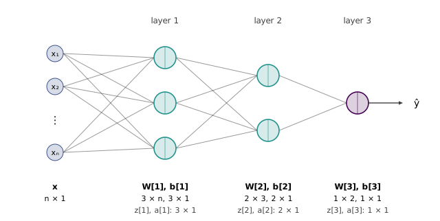
51:31 For the three-layer cat network, pushing one example from input to output is six lines, each layer a linear part and an activation:
This is forward propagation. Where Section 10.2 wrote one equation per neuron, these write one per layer: stacks the three neurons’ weight rows into a matrix, and the sigmoid is applied entry by entry.
53:13 The shapes follow from two facts, that has one entry per neuron in layer and that must turn the previous layer’s activations into it. So is and is , which forces to be ; is and is , so is , one entry per edge between the layers; and is . In general is and is , where is the width of layer . Katanforoosh’s advice is to know every shape in the network before writing a line of code, and it is the tool that makes the next chapter’s derivatives come out right.
10.7 Vectorising over a batch
54:59 Recall the two ends of gradient descent from Section 2.6: stochastic gradient descent updates after every example, with a noisy direction; batch gradient descent updates after seeing all of them, with an accurate one. Either way, a network with many layers does a lot of arithmetic per example, and the way to make that fast is to process many examples in one set of matrix operations rather than in a loop.
55:59 Stack examples as the columns of an matrix , using round-bracket superscripts for the example and square brackets for the layer. Then the first layer for the whole batch is
and is , its -th column the of example . is still : 59:21 feeding the network a thousand images does not give it more parameters. 59:36 But that leaves Equation 10.7 adding a matrix to a vector, which is not defined. The fix is broadcasting: read as the matrix whose columns are all , so the same bias is added to every example. NumPy does this automatically when the shapes are compatible. The generator checks that the broadcast batch computation gives column for column what the per-example loop gives. The remaining lines of Equation 10.6 become capital-letter versions in the same way; the lecture leaves writing them out, with their shapes, as an exercise.
Two student questions in this stretch are worth keeping. 1:03:05 One asks how this differs from principal component analysis, which also builds new features from the inputs. PCA is unsupervised: it finds the directions along which the inputs vary most and never looks at a label. The hidden layer is trained to predict , and a direction of large input variance that does not help with that is of no interest to it.
1:05:53 The other asks how to choose the number of layers and neurons. Nobody knows in advance, so the honest answer is to train several architectures and compare them on the validation set, as in Section 8.4. Experience narrows the search: a harder problem needs more data and a deeper network, and judging which problem is harder is a skill. Telling cats from non-cats seems harder than telling day from night, since cats come in many breeds and nights do not, though even day or night has its trap, a photo taken indoors next to a small window.
10.8 The cost, and why backpropagation starts at the end
1:09:06 With the architecture fixed, what is left is to find its parameters . The objective over a batch is the average loss,
with the logistic loss of Equation 10.2. The lecture keeps the words apart: the loss is the error on one example, the cost the average over a batch. 1:11:13 Differentiation is linear, so the gradient of is the average of the gradients of the per-example losses, and it is enough to work out derivatives of and average at the end. The generator confirms this numerically.
1:12:55 Gradient descent then updates every layer,
which needs six derivatives. 1:14:13 Asked which to compute first, the room suggests , and Katanforoosh argues for . It is the closest to the loss, so its effect on passes through the fewest functions, while affects through every layer above it. Splitting the derivative along the chain of the forward pass,
every factor is easy, and the first two together are . 1:17:33 The next layer down needs exactly that quantity again:
so it is computed once and reused, and the same happens one layer further down with . That is the whole idea of backpropagation: start at the loss, apply the chain rule one layer at a time, and carry the error backwards instead of recomputing it. 1:18:42 The forward equations say which path the chain must take. depends on only through , so the chain for runs through and not through , which is a dead end. The derivation, with the shapes that make the products well defined, is the first half of Section 11.1 in the next chapter.
cs229-notes-deep_learning, section 1, builds the network from the housing example; section 2 vectorises the output computation and the computation over training examples; section 3.1 counts the parameters of the three-layer network () and explains why they cannot all start at zero. The backpropagation derivation is in section 3 and in the separate cs229-notes-backprop.