14 EM Algorithm and Factor Analysis
Lecture 14
EM algorithm, mixture of Gaussians, factor analysis, multivariate Gaussian, coordinate ascent
Lecture video: Lecture 14: EM Algorithm and Factor Analysis · 1:19:48
Based on the lecture by Andrew Ng — CS229, Stanford University, Autumn 2018.
Factor analysis is a density model for data with many more dimensions than examples. For example, a hundred temperature sensors give a hundred-dimensional reading, but you may have only thirty days of data. An ordinary Gaussian cannot be fitted to such data, because its maximum-likelihood covariance is singular. The model assumes that each observation is a low-dimensional hidden cause , mapped linearly into the high-dimensional space, plus independent noise in every coordinate. Because is hidden, the model is fitted with EM, and doing so means working out the conditional distributions of a joint Gaussian.
The lecture first closes off the previous one. It shows how the abstract E- and M-steps of Section 13.7 become code for the mixture of Gaussians, and it recasts EM as coordinate ascent. It then spends the rest of the hour on factor analysis.
14.1 From the general algorithm to the mixture updates
3:00 The general M-step says to maximise the lower bound over with the held fixed. For the mixture of Gaussians, is the responsibility that the E-step computes and stores. The joint density factorises as . So the quantity the M-step maximises is a double sum that can be written out in full:
Ng’s point is that this objective is what gives you the updates. The rule “move each mean to the weighted average of the points” was an intuition in the last lecture, and here it is derived. Differentiating Equation 14.1 with respect to and setting the result to zero gives
and the same procedure gives .
For , “differentiate and set to zero” does not quite work, and the board skips over why. The only terms in are , whose derivative with respect to is . That derivative is positive for every value of , so it never vanishes. Taken alone, the objective wants every to be infinite. What stops it is the constraint , so the step needs a Lagrange multiplier. With the multiplier, the solution is . The generator confirms this on a three-component one-dimensional mixture. At the closed-form M-step, the unconstrained derivative equals exactly for all three components (the multiplier), and none of 300 random perturbations of that stay on the simplex raises .
14:11 Ng then gives a second view of EM that the factor-analysis derivation leans on. Treat the lower bound as a function of both arguments,
The E-step maximises over with fixed, and the maximum is the choice that makes . The M-step maximises over with fixed. EM is therefore coordinate ascent on : it maximises over one block of variables, then the other, and alternates. This view also tells you how to check that an implementation is working. cannot decrease in either step, and since it equals after every E-step, the log-likelihood you print at each iteration must not decrease either. If it ever goes down, there is a bug. On the mixture above, the generator asserts that after each E-step to , and that never falls over 40 iterations: from it reaches after three iterations and at the end.
When is continuous, as it will be in factor analysis, every step of the derivation in Section 13.7 goes through with the sum over replaced by an integral. Jensen’s inequality does not care which kind of expectation it is applied to.
14.2 Fewer examples than dimensions
17:46 A mixture of Gaussians suits data like Ng’s two-dimensional picture with a hundred points: , and each cluster has plenty of points to estimate its covariance. Factor analysis is for the opposite regime, where or . Ng’s running example is a Stanford PhD student’s project with temperature sensors placed around campus buildings: a hundred sensors and thirty days of readings, so and . The goal was anomaly detection by density estimation, as in Section 13.3. A window left open on a winter day produces a reading with low , and in practice the point was saving energy rather than detecting fires. To do this you need a joint density over all hundred sensors, because neighbouring sensors are strongly correlated, and you have thirty examples to fit it with.
22:01 The obvious model is a single Gaussian with its maximum-likelihood estimates and . If , this is singular. The reason is that it is a sum of rank-one matrices whose vectors sum to zero, so its rank is at most . The generator checks the exact statement on random data for and every from 2 to : the rank is , so the estimate is invertible exactly when . A singular breaks the density in two ways. The normaliser contains and the exponent contains , which does not exist, so evaluating gives at best. Ng’s picture with shows the second problem (Figure 14.1, first panel). The fitted Gaussian has its contours squashed to zero width along the segment joining the two points. All of its probability mass lies on that line, so any test point slightly off the line gets density zero. That is a numerical failure, and it is also a bad model of the data.
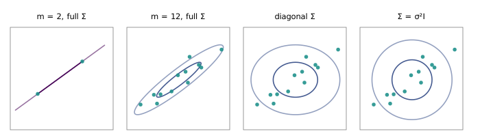
26:53 Ng adds that one of the earliest applications of factor analysis had the same shape: psychological testing, with a hundred questionnaire items and thirty subjects, where the question is how attributes like verbal and mathematical ability are correlated.
14.3 Restricting the covariance
28:15 One way out is to fit fewer parameters. If is constrained to be diagonal, the maximum-likelihood estimate is what you would guess: each feature gets its own sample variance, . That makes parameters in place of about , and they can be fitted from any . The contours are axis-aligned ellipses. The price is that the model assumes the features are uncorrelated, and for a hundred sensors in one room that is plainly false (Figure 14.1, third panel).
31:36 A stronger restriction is , with one parameter and circular contours. Its estimate is the average squared deviation over every coordinate of every example, which is the mean of the diagonal model’s variances. A student asks why anyone would bother with a model that is worse still. Ng’s answer is that it is a building block: factor analysis uses a diagonal covariance for its noise, not for the data.
34:38 Another student asks about the standard fix, a Wishart prior on . In practice this means adding a constant to the diagonal of the maximum-likelihood estimate. Ng’s verdict is that it removes the singularity “in a technical way” but is not the best model for many data sets. The generator puts that verdict to a test at the end of the chapter (Section 14.6). What Ng wants instead is a model that captures the main correlations, such as the room warming and cooling as a whole or one side heating up under the lamps, without paying for a full covariance matrix.
He follows this with an aside about small data that is worth keeping. The large technology companies, he says, all work on the same few big-data problems (translation, speech, face recognition), while many real applications in healthcare and manufacturing have a hundred or a thousand examples. The best algorithm for a thousand examples is often not the best for a million, and the field does not yet know how to make one algorithm work along the whole range. He mentions using a modified factor analysis on a manufacturing problem that same week.
14.4 The factor analysis model
40:32 Like the mixture of Gaussians, the model is a joint density with hidden. This time is continuous and of lower dimension than :
with and independent. The parameters are the mean , the factor loading matrix , and a diagonal . Equivalently, .
43:30 Ng’s reading of the model uses the room. Suppose three strong forces drive the temperatures in the room: the temperature outside, the lights on the left side, and the lights on the right. Then , and holds those three numbers. Each sensor reads a linear combination of the three, weighted by where it sits, so a sensor near the door leans on the outdoor term. On top of that each sensor adds noise of its own, such as a gust of wind or a bad thermistor. The assumption that is diagonal says that this noise is independent across sensors once the shared factors are accounted for. All correlation between sensors has to come through .
46:21 The lecture’s example makes this concrete with , , , , and (Figure 14.2). Seven draws of fall on the real line. Multiplying by places them on the line in the plane. Around each of these points, the noise has axis-aligned elliptical contours, taller than wide in the ratio . Drawing one sample from each gives the observed points. Only those crosses are data. The values, and the points on the line, are latent.
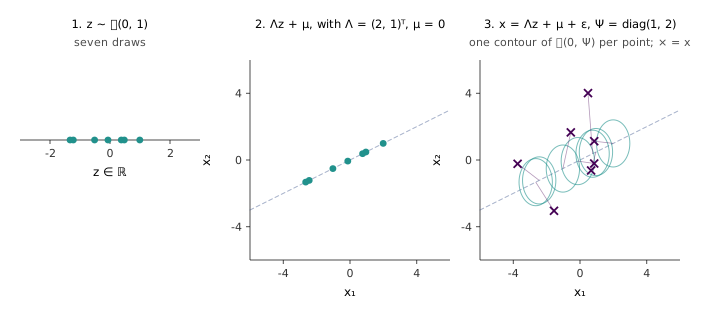
51:05 Ng repeats the construction with and , carrying the five sampled points on a sheet of cardboard and holding it up into three-dimensional space. The data then lie close to a two-dimensional “pancake” in , with some fuzz off it. Factor analysis takes data in a hundred dimensions and models it as lying near a three-dimensional subspace, plus independent noise in each coordinate. 54:57 Asked what happens when the data do not lie near a subspace, he concedes that the model is then not the best one. He adds that in a hundred dimensions you rarely know, because you cannot look.
14.5 Marginals and conditionals of Gaussians
56:43 Fitting the model needs two facts about multivariate Gaussians. Partition a Gaussian vector into blocks and :
The first fact is that the marginal of is . You can prove it by integrating out of the joint density, but the result is the obvious one: the mean and covariance of are the corresponding blocks. The second fact is that the conditional is also Gaussian,
This one is less obvious, and the lecture states it without proof. The conditional mean is a linear regression of on . The conditional covariance does not depend on the value of that was observed.
1:02:32 Applying this to factor analysis starts with the observation that is jointly Gaussian, since is a linear function of the Gaussians and . Its mean is . Ng derives the lower-right block of the covariance and leaves the others to the notes. Expanding
Here the cross terms vanish because and are independent with mean zero. The same expansion gives , so
For the lecture’s example, Equation 14.4 gives the covariance of as rows , and . A Monte Carlo estimate from 200,000 samples in the generator agrees to within 0.015 in every entry.
By the marginal rule, . This explains why the model escapes the singularity: is diagonal with positive entries, so is positive definite however small is. The covariance has free parameters: a rank- part that carries the correlations, plus a diagonal part. 1:10:09 The log-likelihood is perfectly well defined, but setting its gradient to zero has no closed-form solution in and . That is why the lecture turns to EM.
14.6 EM for factor analysis
1:11:03 In the mixture of Gaussians, was a list of numbers. Here is continuous, so the question is how to represent in a computer. The answer is that is Gaussian, by Equation 14.3 applied to Equation 14.4, so it is stored as a mean vector and a covariance matrix:
The generator checks Equation 14.5 against Bayes’ rule applied directly, multiplying the prior on by the likelihood of on a grid of 12,000 points. For three different observations in the lecture’s example, the two agree to in mean and variance. As the formula says, the posterior variance is the same for every observation: . In code, the inverse is avoided with the matrix-inversion lemma, , which is .
1:13:39 The M-step derivation is long, and Ng gives only its two tricks. The first is to recognise expectations instead of expanding integrals. The objective contains terms like . Substituting the Gaussian formula for and integrating is the wrong approach. The integral is , which is , already computed in the E-step. 1:18:13 The second is to expand a Gaussian density when a logarithm sits in front of it. Then the log cancels the exponential and leaves a quadratic in the parameters, whose expectation under is again a quadratic that can be maximised in closed form. The resulting update for is
with the sample mean. is the diagonal of a similar expression, given in the official notes. Equation 14.6 has the form of the normal equations for regressing on , except that the unknown are replaced by their posterior moments. The bracket in the second factor is under . That is the mean’s outer product plus the posterior covariance, because is not .
The official notes warn that dropping here is a common mistake, which treats the posterior mean as if it were the true . They do not say what the mistake costs, so the generator runs both versions (Figure 14.3). The data are 30 examples in dimensions, drawn from a three-factor model; the sample covariance has rank 29, as Section 14.2 says it must. Correct EM increases on every one of 200 iterations, from at the start to after 10 iterations and at 200. Over the last 50 iterations it is still gaining 1.3 nats. The shortcut version is deceptive. It climbs faster at first and reaches at iteration 4, ahead of the correct algorithm. Then the likelihood falls on every remaining iteration, 196 of 200 in all. Correct EM overtakes it at iteration 38, and the shortcut finishes at . The shortcut is not coordinate ascent on any bound, so the monitoring rule of Section 14.1 is exactly what catches it: an implementation whose log-likelihood ever decreases has a bug, even if its first few iterations look better than the correct one.
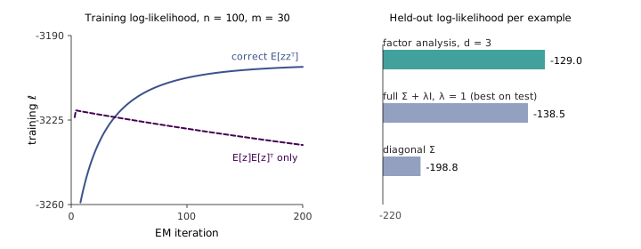
The same run tests Ng’s remark about the Wishart fix from Section 14.3. On 300 held-out examples, factor analysis scores an average log-likelihood of per example. The full Gaussian with added scores , even though was chosen from a grid using the test set itself, which is an unfair advantage. The diagonal Gaussian scores . The comparison does favour factor analysis, because the data were generated from a factor model. What it shows is narrower than “factor analysis is better” in general. When the correlations really are low-rank, adding makes the covariance invertible without capturing that structure, and the diagonal model throws the correlations away entirely.
Restrictions on , the marginal and conditional formulas with a derivation of the conditional, the joint distribution of , and the full M-step for , and are in cs229-notes9, sections 1 to 4. The mixture-of-Gaussians M-step with the Lagrange multiplier for , and the coordinate-ascent view of EM, are in cs229-notes8, sections 2 and 3. The EM algorithm for factor analysis was given by Rubin and Thayer (1982).