11 Backprop and Improving Neural Networks
Lecture 11
backpropagation, activation functions, weight initialization, vanishing gradients, mini-batch gradient descent, momentum
Lecture video: Lecture 11: Backprop and Improving Neural Networks · 1:16:38
Based on the lecture by Kian Katanforoosh — CS229, Stanford University, Autumn 2018.
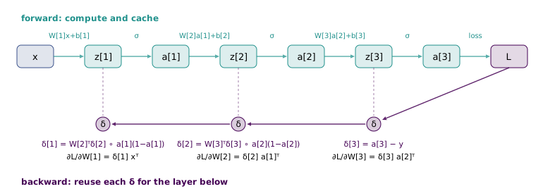
Backpropagation is the chain rule applied one layer at a time from the loss downwards, with each layer’s intermediate result handed to the layer below instead of being recomputed. For the three-layer network of the previous chapter it comes down to one recurrence: the error at the output is prediction minus label, and each layer’s error is the next layer’s error carried back through the transposed weights and multiplied entry by entry by the slope of the activation. The first third of the lecture derives that by hand. The rest is about why a network that computes its gradients correctly can still fail to train, and the standard remedies: the choice of activation, normalised inputs, initial weights of the right size, mini-batches and momentum.
The lecture continues the previous one, again given by Kian Katanforoosh, on the same running example: a colour image flattened into , a layer of three sigmoid neurons, a layer of two, and one sigmoid output that says whether the image shows a cat (Section 10.6).
11.1 The gradient at the output
5:41 The cost is the average of the per-example logistic losses, and since differentiation is linear it is enough to differentiate one loss and average at the end (Section 10.8). Write the loss for one example with the output layer spelled out,
and differentiate with respect to , the parameter closest to it. Each term is a logarithm of a sigmoid of a linear function, so the chain rule gives three factors: from the logarithm, from the sigmoid, whose derivative is , and the derivative of with respect to . The second term is the same with and a minus sign. 15:46 The sigmoid factors cancel against the logarithm’s, the cross terms cancel against each other, and what is left is
The result “doesn’t look that bad,” as Katanforoosh puts it, and it is the same prediction-minus-label form as logistic regression (Equation 10.5), with the activations of the layer below standing in for the input.
12:05 A student asks where the transpose comes from. The answer is a shape argument, and it is the tool for the rest of the derivation. is a scalar and is , so the derivative of one with respect to the other has one entry per entry of and must be as well. In scalar calculus the derivative of with respect to is ; here is , which is the wrong shape, so the answer has to be . Either learn the matrix-calculus identities by heart, or learn to check shapes. The bias works the same way and gives . Averaging over a batch, the cost’s gradient is , which in the matrix notation of Section 10.7 is the single product : the sum over examples is done by the matrix multiplication.
11.2 The chain rule, one layer down
19:05 For the lecture does not start over. It decomposes the derivative along the path that connects to the loss in the forward equations:
20:24 The path has to go through . also depends on and , but differentiating with respect to those leads nowhere: they do not depend on , and the error has to travel through variables that do. 22:04 Asked which part of this is already known, a student says the first three factors and then corrects it to two, which is right: since , Equation 11.1 says . The remaining factors are each one step of the forward pass. is the sigmoid’s derivative, ; brings in as before; and 25:24 is or its transpose, which the shapes decide: is a scalar and is , so the factor is the vector .
28:01 Written in the order the chain rule produced them, the factors are , , and , and they do not multiply. The derivation so far was a bookkeeping of which quantities appear, not of how they combine. Two facts put them together. The sigmoid acts on each entry of separately, so its derivative enters as an entry-by-entry product, written , and that is true of every activation. And the result must have the shape of , , which fixes the order of the rest:
Inside the parentheses is a vector, , and the outer product with the vector gives . The lecture leaves as an exercise; it comes out the same way, and the pattern is worth stating once in general. Write for the error at layer of an -layer network with activation . Then
with . The first equation holds for a sigmoid output with the logistic loss and for a softmax with cross-entropy alike. The generator implements exactly these four lines for the 3-2-1 sigmoid network and compares every one of its parameters’ gradients with finite differences on fifty random networks; the worst disagreement is .
31:21 Katanforoosh’s view is that hardly anyone derives these by hand any more, since programming frameworks differentiate automatically, but that it is worth having done once, both to understand what the framework is doing and to read papers that write gradients out. For the rigorous version he points to the lecture notes.
11.3 What the forward pass must keep
32:04 Every factor in Equation 11.3 other than itself is something the forward pass already computed: the activations , the values depend on, and the weights. Discard them and the backward pass would have to re-run the forward pass from each time it needed one, going forwards again to reach , then again to reach . So the forward pass caches what it computes and the backward pass reads it. This is a trade of memory for computation, and the memory is not small: every activation of every layer for every example in the batch is held until the backward pass reaches it.
11.4 Activation functions
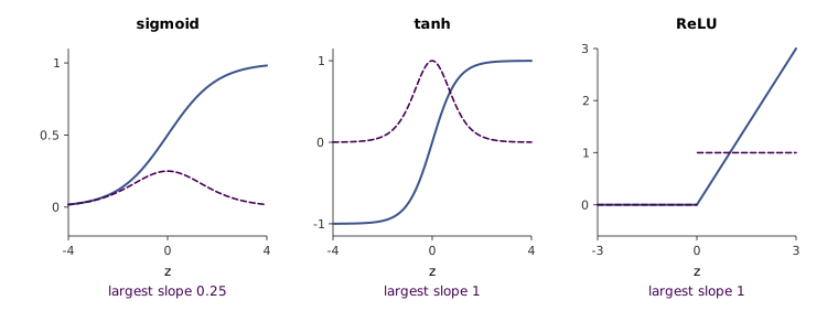
34:44 Getting the gradients right is necessary and nowhere near sufficient; a network built and differentiated correctly usually still trains badly, and the rest of the lecture is the set of practical fixes. The first is the choice of activation. There are three in common use:
with derivatives , , and the indicator . 37:08 The sigmoid’s strength is that its output reads as a probability. Its weakness, which a student names, is saturation: for large positive or negative the curve is flat, its derivative is nearly zero, and since that derivative is a factor in every below it, layers early in the network get almost no gradient and barely move. The derivative is small even at its best. Its maximum is , at , so every sigmoid layer shrinks the gradient passing through it by at least a factor of four, and ten of them shrink it by at least , about a million. tanh saturates in the same way at both ends, but its slope at the centre is 1 and its output is centred on zero.
38:52 ReLU does not saturate for positive inputs: its slope there is exactly 1, so it passes the gradient through unchanged rather than scaling it down. Its slope for negative inputs is exactly 0, which has its own cost the lecture does not get to: a ReLU neuron whose input is negative for every example receives no gradient at all and stops learning. That trade has worked out well enough that ReLU is the usual choice for hidden layers.
39:53 For the output layer the choice is made by the range of what is predicted, not by trainability: a sigmoid for a probability in , tanh for values in such as the rewards of reinforcement learning, a ReLU for a non-negative quantity such as a house price, the identity for an unrestricted one. 45:18 Within a hidden layer the convention is one activation for every neuron, so that a layer is described as, say, a fully connected ReLU layer. People have tried mixing activations inside a layer without finding a reason to, and the choice is treated as a hyperparameter like any other, settled by experiment rather than by theory.
11.5 Why the network needs a non-linearity
41:06 A student asks why these particular functions, and Katanforoosh answers by taking the activation away. With the identity in every neuron of the 3-2-1 network the forward pass substitutes into itself:
43:52 Three layers of parameters compute exactly what one layer computes, an affine function , and adding layers changes nothing: however deep, the network is a linear regression. The capacity of a network to represent complicated functions comes entirely from its activations. The lecture’s phrasing is that any function but the identity will do; strictly, the problem is any affine activation, since collapses in the same way, and what is needed is a non-linear one. The generator confirms the collapse on random inputs to machine precision.
11.6 Normalising the inputs
48:16 If the inputs are large, is large and the sigmoids saturate before training starts. The simple remedy is to standardise the inputs using the training set: compute the mean and variance of each feature,
entry by entry, and replace every by . Subtracting centres the cloud of points on the origin; dividing by gives every feature the same spread.
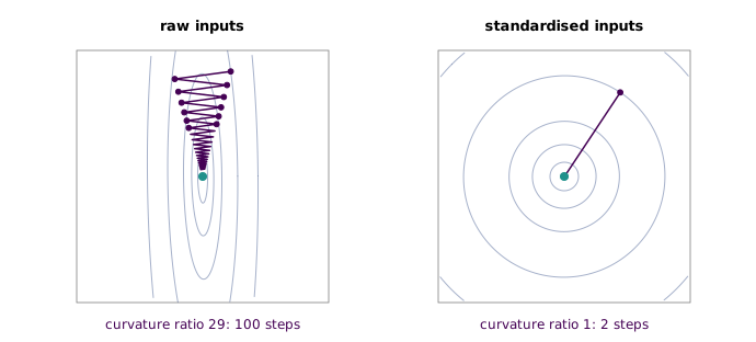
51:18 The second reason is the shape of the cost. When features have very different scales, or sit far from zero, the cost is a long narrow valley in parameter space, and gradient descent, which moves perpendicular to the contours, crosses the valley again and again while making slow progress along it. After standardising, the contours are closer to circles, the gradient points nearly at the minimum, and descent goes almost straight there. Figure 11.3 makes the comparison on a least-squares problem with two features, one centred at 2 and the other on a small scale. The ratio of the cost’s curvatures along its two axes is 29 with the raw inputs and 1 after standardising, and gradient descent, each run at its best fixed learning rate, needs 100 steps against 2. Standardising equalises scales, not correlations: afterwards the curvature matrix of a least-squares cost is the features’ correlation matrix, so two strongly correlated features still leave a long valley, tilted at 45°, which decorrelating transforms such as the PCA of a later chapter address.
53:03 One rule matters more than the formulas: and are computed on the training set and then reused, unchanged, on the dev and test sets. The network has learned to expect inputs transformed in one particular way, and normalising the test set by its own statistics would feed it a differently transformed input.
11.7 Vanishing and exploding gradients
54:19 To see why depth makes all of this harder, take a network of ten layers with two neurons each, identity activations and zero biases. The output is then the input multiplied by every weight matrix in turn,
56:05 If every is a little larger than the identity, say , the product is , which for is about ; if every one is , it is . Small departures from 1 compound geometrically. 57:16 The same products appear in the backward pass, because Equation 11.3 multiplies by and by once per layer, so the gradients reaching the early layers either explode or vanish. With sigmoids the factors alone contribute at most each (Section 11.4). Nothing in the gradient computation is wrong; the arithmetic is simply unforgiving over many layers.
11.8 Initialising the weights
58:24 The lecture’s goal is to keep each layer’s multiplier “close to 1”, which needs a little care, because that is a statement about the layer and not about individual weights. A neuron computes , a sum of terms, and the more inputs it has, the larger gets unless the weights shrink to compensate. Make that precise: if the weights and inputs are independent with mean zero, then
so has the same variance as its inputs when , or standard deviation . The lecture’s code multiplies standard normal draws by , where is the number of inputs to layer . The generator checks the variance identity by simulation, getting against .
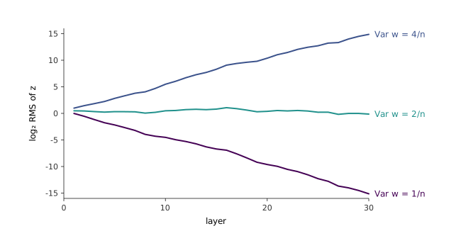
1:02:07 Katanforoosh reports, as an empirical observation, that a ReLU network trains better with in place of . There is a clean reason, given by He et al. (2015): a ReLU zeroes the negative half of a symmetric input, which halves the mean square of what it passes on, so the variance needs to start twice as large to come out the same. Figure 11.4 shows how quickly this matters. In a 30-layer ReLU network with weights of variance , the signal loses half its mean square at every layer and ends about of its starting size; with it grows by the same factor; with it stays level.
1:02:38 The lecture then presents “Xavier initialisation” and “Glorot initialisation” as two different schemes. They are one person’s name: the method is from Glorot and Bengio (2010), whose first author is Xavier Glorot. The paper asks for two things at once, that activations keep their variance going forwards, which needs , and that gradients keep theirs going backwards, which needs . Both cannot hold unless the layer is square, and the compromise it proposes is
the reciprocal of the arithmetic mean of the fan-in and fan-out (the lecture says a geometric average). This is the formula the official notes give, under the name “Xavier/He”, though He’s is a different rule for a different activation. Glorot and Bengio derived theirs for tanh-like units; for ReLU networks, He’s is the one that holds the variance.
1:04:02 Finally, the initial weights must be random, and not merely small. If all the weights of a layer start equal, every neuron in it computes the same function, receives the same gradient, and is updated identically, forever: the layer behaves as a single neuron, however wide it is. The generator trains the 3-2-1 network from equal weights for 6,000 steps of stochastic gradient descent, and the three hidden neurons’ weights end up identical to the last bit. Starting from zero is the extreme case, and the official notes work it through. Random initial values break the symmetry, so that the neurons start in different places and can learn different things; biases have no such problem and can start at zero.
11.9 Mini-batch gradient descent
1:05:16 The two versions of gradient descent seen so far sit at opposite extremes. Batch gradient descent vectorises well but makes one update per pass through the data, and with a million images one update is very slow. Stochastic gradient descent updates after every example, quickly but noisily, and gives up vectorisation. Mini-batch gradient descent takes the middle. Split the training set into batches, written with curly braces, , of 1,000 examples each, and loop:
- pick a batch ;
- forward-propagate the whole batch and compute its cost ;
- backpropagate to get the gradients of ;
- update and for every layer.
Each update is a matrix computation over a thousand examples, which a GPU does at once, and a thousand examples already give a useful estimate of the direction to move in. 1:09:30 The price is noise. Plotted against iterations, the cost of batch gradient descent falls smoothly, while that of mini-batch descent falls on average but wobbles, since each step follows one batch’s estimate of the gradient. The smaller the batch, the larger the wobble, and quantitatively: for batches drawn at random, the variance of the gradient estimate is inversely proportional to the batch size. On a toy regression the generator measures 9.9, 0.98 and 0.10 for batches of 1, 10 and 100.
11.10 Momentum
1:11:24 Return to the long narrow valley of Section 11.6. Gradient descent zig-zags across it because the steep direction dominates every gradient, and the useful step would be large along the valley and small across it. Momentum gets there by looking at the history of updates. 1:13:27 Averaged over a few steps, the components across the valley alternate in sign and cancel, while the components along it all point the same way and add up. Stepping along the average rather than the latest gradient damps the zig-zag and builds up speed along the floor. In the lecture’s form,
where , the velocity, is an exponentially weighted average of past gradients, and , often around 0.9, sets how long a memory it has. 1:15:42 It costs one more line of code and one more variable per parameter. The physical picture is a heavy ball rolling downhill: its velocity cannot reverse at every bump, and plays the part of friction.
A computation sharpens the picture in a way the lecture does not. In this form, at the same learning rate as gradient descent, momentum helps only modestly: on a quadratic 100 times steeper across the valley than along it, gradient descent at its best fixed rate takes 346 steps to converge and momentum with at that rate takes 272. The large gain comes from what momentum makes possible. Gradient descent diverges as soon as exceeds , here , while the averaging raises the limit to , here . At , three times the rate that makes gradient descent blow up, momentum converges in 90 steps.
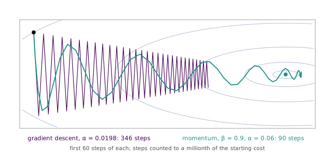
1:15:58 The optimisers used most in practice, RMSProp and Adam, go further and give every parameter its own effective learning rate, scaled by a running average of its squared gradients. Adam combines that scaling with momentum. The lecture’s closing point about them is a sociological one: a new optimiser has to prove itself across a wide range of problems before people adopt it, which is why so few are in common use.
cs229-notes-backprop derives the backward recurrence for a network of any depth, with the matrix calculus the lecture replaces by shape analysis. cs229-notes-deep_learning, section 3, covers backpropagation for the three-layer network; section 3.1 the parameter count, why zero and equal initialisations fail, and the variance-scaled initialisation; section 3.2 stochastic and mini-batch gradient descent and momentum; and section 3.3, which the lecture did not reach, L2 regularisation and parameter sharing.