5 GDA and Naive Bayes
Lecture 5
generative learning algorithms, Gaussian discriminant analysis, naive Bayes, Bayes’ rule, spam filtering
Lecture video: Lecture 5: GDA and Naive Bayes · 1:18:52
Based on the lecture by Andrew Ng — CS229, Stanford University, Autumn 2018.
Every algorithm so far has been discriminative: it models directly, or maps to a label, and learns by searching for a boundary between the classes. This lecture introduces the other family. A generative learning algorithm models what each class looks like, , together with how common each class is, , and classifies a new example by asking which class model it fits better. Gaussian discriminant analysis (GDA) does this with a Gaussian per class and turns out to imply exactly the logistic form of lecture 3 — but with stronger assumptions, which help when data are scarce and hurt when they are wrong. Naive Bayes does it for text, with one binary feature per word and an assumption Ng calls flatly untrue, and still makes a serviceable spam filter.
5.1 Two ways to build a classifier
1:09 Ng starts from the tumour data again, two features and two classes. Logistic regression initialises a line and lets gradient descent move it until it separates the malignant from the benign examples; it is searching for a boundary. A generative algorithm never looks for a boundary. It takes the malignant tumours alone and fits a model of where they live — roughly inside one ellipse — then does the same for the benign tumours. When a new patient arrives, it compares their features against the two models and picks the class whose model the patient resembles more.
3:56 In symbols, a discriminative algorithm learns , or a function from to labels. A generative one learns — what the features are like given the class — and the class prior , the odds that a tumour is malignant before the patient has even been examined. 5:50 Bayes’ rule converts those two into the quantity a classifier needs:
35:49 If all that is wanted is the most likely label, the denominator can be skipped. does not depend on , so
and implementations often never compute at all. Ng’s aside on notation is worth keeping: is , the smallest value attained, while is , the input that attains it.
5.2 The multivariate Gaussian
9:46 GDA needs a Gaussian over vectors. A random vector is distributed , with mean vector and covariance matrix , symmetric and positive definite, if its density is
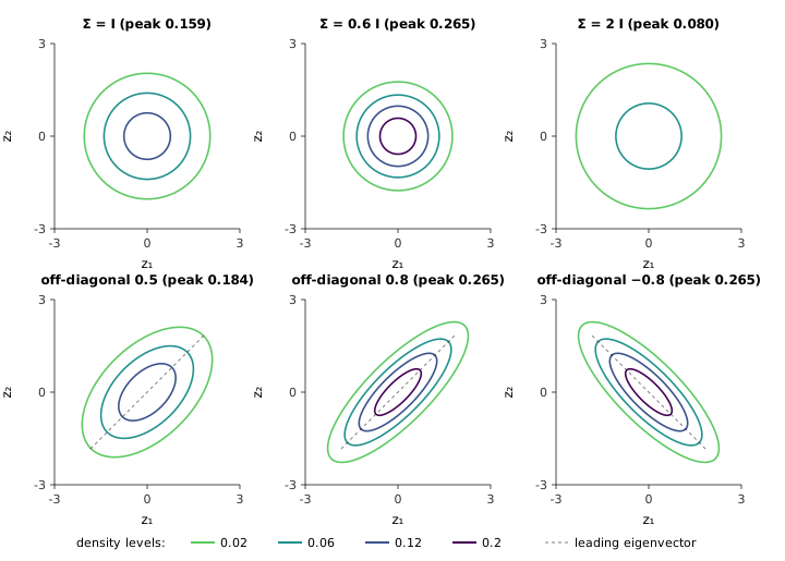
where . Ng’s view is that almost nobody memorises this formula until they have used it enough times, and that pictures teach it better. 12:00 Ng projected a sequence of three-dimensional plots; Figure 5.1 recomputes them as contour maps, every panel at the same four density heights so that panels can be compared.
figures/05-gda-naive-bayes/make_diagrams.py.
With and — the standard Gaussian — the contours are circles. Multiplying by shrinks the spread, and because the density must still integrate to one, it grows taller: in two dimensions the peak scales by , from to . Doubling halves it. Raising the off-diagonal entries makes and positively correlated, and the circles stretch into ellipses along the diagonal, narrower as the entry rises to ; negative entries tilt them the other way. One coincidence in the figure is a useful check on the formula: the off-diagonal- Gaussian has the same peak as , because both have . Changing moves the bump without changing its shape.
16:26 A student asked whether the columns of point in meaningful directions. Ng’s answer is that single columns are not worth reading in isolation — the matrix is symmetric — but its eigenvectors are: they are the principal axes of the elliptical contours, the long axis belonging to the largest eigenvalue. For the off-diagonal- panel the eigenvalues are and , with the long axis along . This is the idea principal component analysis builds on later in the course.
cs229-notes2, section 1.1, defines the multivariate normal and shows the same family of surface plots.
5.3 The GDA model and its fit
19:02 Gaussian discriminant analysis assumes that each class’s features are Gaussian, with a mean of their own and a covariance they share, and that the label is a coin flip:
For generative models Ng drops the convention , so . The parameters are , and . 20:24 A shared is a choice, not a necessity — separate and are perfectly reasonable — and the reason for it becomes clear when the decision boundary is drawn.
23:05 The fit is where the two families part. Logistic regression chose to maximise the conditional likelihood . GDA maximises the joint likelihood,
26:56 Taking logs, differentiating and setting the derivatives to zero gives closed forms — the derivation is a problem-set exercise, and Ng gives the answers along with the intuition for each:
The indicator is 1 when its argument is true and 0 when it is false. The estimate of is the fraction of malignant tumours in the training set, as the maximum-likelihood bias of a coin is the fraction of heads. Each mean is the average of its class’s feature vectors: the indicator in the numerator keeps only that class’s examples, the one in the denominator counts them. And is the average outer product of each example’s deviation from its own class mean — one covariance fitted to both clouds at once. Ng is careful to say that this intuition is not the derivation; the derivation is calculus on . The generator takes the shortcut of checking the result instead: on 80 synthetic points, 500 random perturbations of the closed-form estimates all lower the joint log-likelihood.
There is no iteration anywhere in Equation 5.4: fitting GDA is computing two means and a covariance. That will matter when Ng explains why GDA is still worth using.
The model and its maximum-likelihood estimates are cs229-notes2, section 1.2.
5.4 GDA’s boundary is logistic
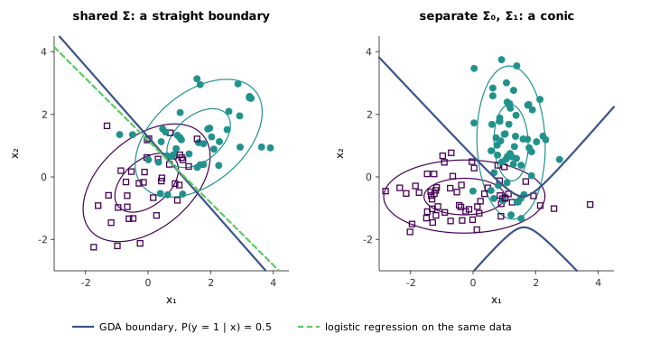
37:07 On the same two-feature data, Ng shows logistic regression’s line migrating over about twenty iterations of gradient descent, then GDA fitting one Gaussian to each class and classifying by Bayes’ rule. Both produce straight boundaries, and the two lines are close but not the same (Figure 5.2, left).
figures/05-gda-naive-bayes/make_diagrams.py.
39:42 A student asked why the model uses two means but one covariance. With a shared the boundary is linear, which is what many problems want. With and the model also works, but the boundary is no longer a line, and Ng says the parameter count roughly doubles. That holds for the covariance part, and for the whole model only when is large: counting and the means too, a shared covariance needs parameters and two covariances , a ratio of at , at and at . 58:13 Asked later what the posterior looks like with separate covariances, Ng’s recollection was that it is still a logistic function, but with quadratic terms inside it. That is right: the log-odds becomes a quadratic in , and its zero set is a conic (Figure 5.2, right).
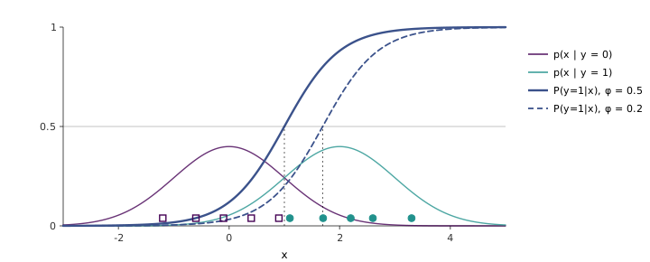
41:02 The connection to logistic regression is the lecture’s most interesting property of GDA. Fix the parameters and, for a single feature, evaluate by Bayes’ rule at point after point along the axis. 43:31 Far to the left, almost any point must have come from the class-0 Gaussian, so the posterior is near 0; far to the right it is near 1; at the midpoint between the two means, Ng says, you cannot tell, so it is . Joining the dots gives an S-shaped curve, and 47:13 it is exactly a sigmoid (Figure 5.3). With a shared covariance the quadratic terms of the two Gaussians’ exponents cancel in the log-odds, leaving
The generator confirms the identity at 200 random points against Bayes’ rule computed directly.
figures/05-gda-naive-bayes/make_diagrams.py.
The midpoint claim holds only when the classes are equally likely. The last term of is the prior log-odds, and it shifts the curve. For one feature the crossing point is
so with means and , unit variance and a prior of on class 1, the boundary moves from to : a rarer class needs stronger evidence. On a malignant/benign problem, where is usually far from one half, this term is anything but negligible.
47:53 So both algorithms end up with a sigmoid in , but they do not end up with the same sigmoid. GDA’s is a byproduct of fitting the joint likelihood; it is not the that maximises the conditional likelihood, which is what logistic regression computes. On the 80 points of Figure 5.2, logistic regression reaches a conditional log-likelihood of , and the GDA implies scores on the same objective. Neither is wrong; they are answering different questions.
5.5 Which one to use
48:57 Ng frames the comparison as an implication that runs only one way. If Equation 5.3 holds, then is logistic — that was the previous section. But assuming that is logistic says nothing about being Gaussian. 53:08 Ng’s counterexample: if and are Poisson with means and , the posterior is again logistic, since the log-odds is , linear in . The same holds, Ng adds, whenever the two class-conditionals are the same exponential family differing only in the natural parameter, with . GDA therefore makes the stronger assumptions and logistic regression the weaker.
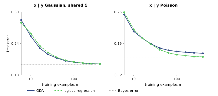
54:46 The principle that follows is one Ng says will recur throughout the course. Stronger modelling assumptions, when they are roughly right, let an algorithm learn from less data, because the assumptions are information it no longer has to extract from examples. When they are wrong, they cost accuracy that more data cannot recover. Weaker assumptions are more robust: if you do not know whether the data are Gaussian or Poisson or something else from the family, logistic regression is correct in all those cases.
Figure 5.4 puts numbers on this. In a world built to satisfy GDA’s assumptions, GDA’s average test error is lower than logistic regression’s from 10 to about 100 training examples, by up to half a percentage point, and both converge to the Bayes error of — though at 6 examples logistic regression, with a slight ridge penalty to keep it finite on separable samples, is ahead. With two features the advantage is real but small; Ng and Jordan (2002) analysed the same trade-off for naive Bayes against logistic regression and found it grows with the number of features: the generative model can approach its (higher) asymptotic error with a number of examples logarithmic in , the discriminative one with roughly linear. In the Poisson world GDA is misspecified, and still it is slightly ahead at 6 and 10 examples — the assumptions are wrong but informative. The curves cross near 25 examples, and from there logistic regression pulls ahead, reaching at 400 examples against GDA’s . With 20,000 examples logistic regression sits at the Bayes error of while GDA stalls at , an error no amount of data removes.
figures/05-gda-naive-bayes/make_diagrams.py.
56:13 Ng’s own practice follows from this. With large datasets, which is most problems now, Ng would usually reach for logistic regression, because data can make up for what the algorithm was not told. There are two sources of knowledge, in Ng’s account: the assumptions you build in and what is learned from data. With plenty of the second you can afford fewer of the first. 56:56 When Ng does use GDA today it is more for computation than accuracy — two means and a covariance, no iterative optimisation.
58:45 Should one test whether the data are Gaussian before using GDA? In practice, Ng says, if you have enough data to run a statistical test and believe it, you probably have enough to use logistic regression. What people actually do is plot the data, rule out GDA if it is obviously non-Gaussian, and otherwise — with, say, fifty healthcare records — use judgment, perhaps by asking doctors whether the distribution is plausibly Gaussian. 59:47 This leads Ng to a broader view: the field has somewhat overhyped big data. More data almost never hurts, but many applications have a hundred examples rather than a million, and there the designer’s skill — including the choice of what to assume — matters far more: on a million-image benchmark many teams do well, while with a hundred examples the skilled teams do much better than the rest. 1:02:42 Asked whether the comparison carries over to more than two classes, Ng says it does, with softmax regression as the discriminative counterpart.
cs229-notes2, section 1.3, makes the same comparison and states that GDA is asymptotically efficient when its assumptions hold.
5.6 Naive Bayes
1:04:08 GDA needs continuous features. Naive Bayes is a generative algorithm for discrete ones, and Ng builds it around spam filtering, though the same method applies to any text classification — the lecture mentions eBay sorting free-text listings into product categories.
1:05:08 The first question is how to turn an e-mail into a feature vector. Take a list of words — conceptually the dictionary, from “a” and “aardvark” to “zymurgy”, in practice the 10,000 most frequent words in your own training set, so that “CS229” makes the list even though no dictionary has it — and set if word appears in the e-mail and if not. So with .
1:09:28 Modelling directly is hopeless: a distribution over all binary vectors needs parameters for each class, a number with 3,011 digits. 1:10:00 Naive Bayes assumes that the are conditionally independent given . The chain rule of probability, which is always true, writes the joint as ; the assumption drops every conditioning variable except ,
In words: once you know whether an e-mail is spam, learning that it contains “buy” tells you nothing about whether it contains “aardvark”. Figure 5.5 shows this as the graphical model Ng sketches for those who have met them.
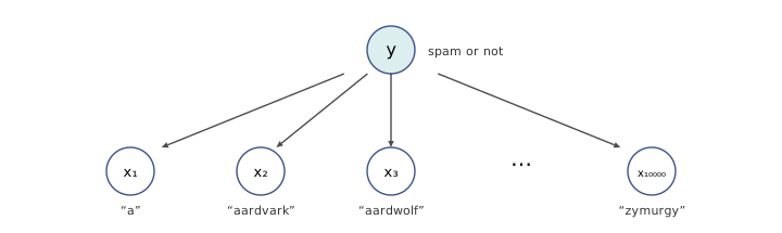
1:11:53 Ng does not defend the assumption as true. It is not, mathematically — words in an e-mail are obviously correlated — but, as with data that are not quite Gaussian, it may be not so wrong that you cannot get away with it. Where it does bite is worth seeing. Suppose a word appears in 60 percent of spam and 10 percent of other mail, and a second feature happens to be an exact copy of it (in real text, a word and its plural, or “click” and “here”). The true posterior from seeing the word, with equal priors, is ; the second feature adds no information, but naive Bayes multiplies its likelihood in again and reports . Correlated features are counted as independent evidence, which makes naive Bayes overconfident even when its decisions are reasonable.
1:13:46 The parameters are , the chance that word appears in a spam e-mail, for non-spam, and the prior — numbers, 20,001 for the 10,000-word vocabulary, instead of a number with three thousand digits. 1:15:00 Maximising the joint likelihood, exactly as for GDA, gives counts:
and the same with . Of all the spam e-mails in the training set, what fraction contain “buy”? That fraction is . Prediction multiplies these numbers by Equation 5.6 and applies Bayes’ rule.
Naive Bayes has the same relationship to logistic regression that GDA has. Its log-odds is a sum over words of terms that depend on only through , so it is exactly linear: with . The generator checks this on every input of a six-word vocabulary. Naive Bayes is a linear classifier whose weights are set by counting rather than by optimisation.
1:17:32 Ng’s verdict is that naive Bayes is “not too horrible”, that logistic regression does better almost all the time, and that naive Bayes is nonetheless very efficient: fitting is counting, prediction is multiplying, and the counts can be updated as new labelled mail arrives without refitting anything. This is the regime Ng and Jordan studied: naive Bayes reaches its own, higher, asymptotic error with fewer examples. 1:18:14 Ng flags one flaw that makes the version above “nearly work”: zeros. If a word never appears in any training e-mail, its estimate is in both classes, an e-mail containing it gets under both, and the posterior is . Even a word seen only in non-spam drives the spam probability of any e-mail containing it to exactly zero, however spammy the rest. The fix, Laplace smoothing, opens the next lecture.
cs229-notes2, section 2, develops naive Bayes for the same spam example; Laplace smoothing (2.1) and the multinomial event model for text (2.2) come with lecture 6.