15 PCA and ICA
Lecture 15
principal component analysis, PCA, eigenvectors, dimensionality reduction, independent component analysis
Lecture video: Lecture 15: PCA and ICA · 1:18:35
Based on the lecture by Andrew Ng — CS229, Stanford University, Autumn 2018.
Principal components analysis (PCA) reduces -dimensional data to dimensions by projecting it onto the directions along which it varies most. Those directions are the top eigenvectors of the data’s covariance matrix. Like factor analysis in the previous lecture, PCA assumes the data lie near a low-dimensional subspace. Unlike factor analysis it has no probabilistic model: it does not define , it just finds the subspace. Ng spends as long on when not to use PCA as on how it works. The last quarter of the lecture sets up independent components analysis (ICA), which looks for statistically independent directions instead of high-variance ones. The algorithm itself is in lecture 16.
15.1 One-dimensional data living in two dimensions
2:09 Ng’s first example is a school that measured its children’s heights twice in the same month, once in centimetres and once in inches, with each value rounded to a whole unit. Plotted against each other, the two numbers lie almost exactly on a line. The data have , but they are really one-dimensional: a child’s height plus a little rounding noise perpendicular to the line. PCA’s job is to find that line, the principal axis of variation, and replace each point by its position along it.
Because centimetres and inches measure the same thing, he offers two less contrived examples. In the first, two vibration sensors made by different manufacturers sit on different parts of a factory machine. Both measure how hard the machine is shaking, which is useful for preventive maintenance, since the vibration pattern changes before a machine fails. 5:50 In the second, from his autonomous-helicopter work, each pilot is scored on skill and on enjoyment of flying. The two might both reflect one underlying aptitude. Going from two dimensions to one is only for the whiteboard. In practice, Ng says, PCA takes something like 10,000 dimensions to 100 or 1,000.
7:29 Before running PCA, the data are standardised. Subtract the mean of each feature, then divide each feature by its standard deviation, so that every feature has mean 0 and variance 1. Section 15.4 explains why both steps matter.
15.2 Two definitions of the best direction
10:00 Ng draws two candidate lines through the standardised height data: the 45-degree line, which is clearly right, and the perpendicular line, which is clearly wrong. He then gives two ways to say what makes the first one right (Figure 15.1). Project every point orthogonally onto a line. For the good line, the projection segments are short, so the sum of squared distances from the points to their projections is small. The projected points are also spread out along the line, while on the bad line they bunch together near the origin. So PCA could be defined as minimising the squared projection distance or as maximising the variance of the projections.
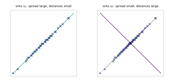
12:00 The two definitions are the same, and the reason is Pythagoras. For a unit vector and a centred point , the squared length of the point splits into the squared length of its projection plus the squared distance to it:
The left side does not depend on . Averaging over the data, projected variance plus mean squared distance is a constant, so maximising one minimises the other. The generator checks this at 3,600 directions around the half-circle. The two terms sum to the same constant to , and the direction with the largest variance is exactly the direction with the smallest distance. On the height data that direction is 45.0°. The projected variance there is 1.9986 and the mean squared distance is 0.0014, out of a total of 2, because the correlation between the two measurements is 0.9986. Ng leaves the proof to the homework and recalls a paper that collected many equivalent derivations of PCA. Historically these two are the founding pair: Pearson (1901) posed the problem as fitting the closest line or plane to a set of points, and Hotelling (1933) posed it as finding components that account for as much of the variance as possible.
15.3 The principal direction is an eigenvector
13:14 Ng derives PCA from the variance definition. For a unit vector , the projection of onto it has length , so the problem is
where is the covariance matrix of the standardised data. Ng apologises that the symbol is the same as the one for summation. 19:13 The maximiser is the principal eigenvector of , the one with the largest eigenvalue. The argument uses a Lagrangian, . Setting its gradient in to zero gives , so any stationary point of the constrained problem is an eigenvector. At such a point the objective equals , so the best eigenvector is the one with the largest eigenvalue, and that eigenvalue is the variance captured. The generator checks this on a random covariance by finding every stationary point of around the half-circle of directions. It finds two, each lies along an eigenvector to within , and the value of the objective there matches the eigenvalue to .
22:11 To keep dimensions, take the top eigenvectors . The new representation of is the vector of its projections onto them:
The second formula decompresses: it maps the numbers back to a point in on the -dimensional subspace. For the heights, is a single cleaned-up estimate of each child’s height, and mapping it back puts every child exactly on the line. Because is symmetric, its eigenvectors can always be chosen orthogonal, so is an orthonormal basis of the subspace. 47:11 A student asks whether the test set needs its own eigenvectors. It does not. The are computed once, on the training set, and the same ones are used to map every future example.
15.4 Pre-processing and the choice of k
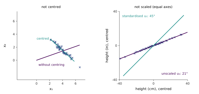
28:07 A student asks why the pre-processing matters, and Figure 15.2 shows both cases. If the data are not centred, is a second moment about the origin, not a covariance. Its top eigenvector points from the origin towards the cloud, not along it. In the generator it lies within 2° of the direction of the data’s mean. If the features are not scaled, a feature measured in small units has numerically large variance and dominates. Ng’s example is centimetres against kilometres. The heights show the effect in a milder form. Centimetre values are 2.54 times the inch values, so the unstandardised principal direction lies at 21.4°, close to . That is the line , which is a statement about units, not about the data. After standardising, the principal direction is at exactly 45°.
58:57 To choose , look at the eigenvalues. Since the eigenvalue is the variance along , the fraction
is the share of the total variance kept by the first directions. Practitioners report choosing to “retain 90%” (or 95, 98, or 99%) of the variance. Ng adds that compressing very high-dimensional data tenfold while keeping 95% of its variance is common. The same quantity measures reconstruction quality. The mean squared error of the decompression in Equation 15.2 equals the sum of the discarded eigenvalues, , so “variance retained” is one minus the relative reconstruction error. The generator asserts this equality for every from 0 to 10 on a ten-dimensional data set.
15.5 When to use PCA, and when not to
31:54 The use Ng endorses most is visualisation: projecting data from dimensions down to 2 or 3 so that it can be plotted. His example is from Krishna Shenoy’s neuroscience lab at Stanford. Monkeys were trained to tap a square on a touch screen when it appeared, in exchange for juice, while about 50 electrodes recorded activity in their brains. A 50-dimensional time series cannot be looked at directly. A former CS229 student in the lab projected it with PCA and could watch the brain’s state move through two or three dimensions: waiting, preparing once the target appeared, holding, and then moving off at the go signal. 36:15 The second endorsed use is compression for efficiency. High-dimensional data usually lie close to a much smaller subspace. Ng calls it “just a fact of life”. Feeding a learning algorithm a 1,000-dimensional in place of a 10,000-dimensional saves memory, bandwidth and compute.
38:23 He calls two other uses questionable. The first is reducing overfitting by shrinking the number of features before, say, logistic regression. In his experience this works about half the time. The half that works gets published and the half that fails does not, so the literature makes it look more reliable than it is. He uses regularisation for this instead. 40:16 The second is measuring similarity in a reduced space. In early face recognition, two images were compared by Euclidean distance after PCA rather than in raw pixel space, in the hope that the projection would remove noise. Sometimes it helps a little, but not reliably. 42:11 This was the era of eigenfaces. Researchers ran PCA on face images and plotted each eigenvector as a picture. Then they read meaning into individual eigenvectors: one is the lighting direction, another is a beard. Ng’s judgement is that such readings were “at least as much a product of the researcher’s imagination” as of the data. The reason is that individual eigenvectors are unstable, which the next section quantifies.
44:35 His rule of thumb follows: before putting PCA into a system, try the system on the original . Class project proposals often include a PCA step by default. Unless you need the speed or the memory, the step adds a component to debug without a reason. Asked whether there is a minimum dimension below which PCA is pointless, he says no. Even going from two dimensions to one is justified if halving memory really matters.
15.6 Why individual eigenvectors should not be interpreted
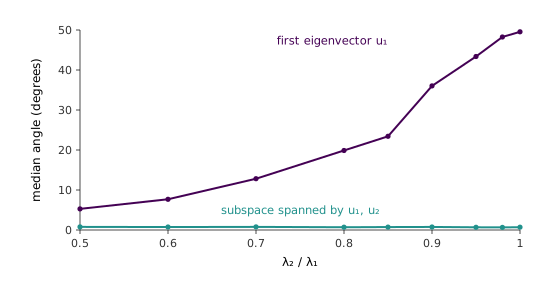
54:49 A student asks why k-means centroids are treated as interpretable and principal components are not. Ng’s answer is that individual eigenvectors are numerically unstable, while the subspace spanned by the first of them is stable. His picture is three-dimensional data lying close to the plane of the whiteboard. and are two directions in that plane, and points out of the board. A small change to the data can spin and around inside the plane, while the plane itself stays put. He says that changing one training example “in the fifth decimal place” can change the eigenvectors significantly.
That claim is true only under a condition the lecture leaves implicit. How far an eigenvector moves depends on the size of the perturbation relative to the gap between its eigenvalue and the next one. The generator tests it with data whose top two eigenvalues differ by an exact relative gap. The data are a regular twelve-sided polygon in a plane, stretched slightly along one axis, plus two points off the plane. Changing one coordinate of one point by moves by when the gap is , when it is , when it is , and when it is . The plane spanned by moves by less than degrees in every case. So a fifth-decimal change matters only when the eigenvalues agree to about five decimals.
The more realistic version is the one Ng gives in answer to a follow-up question 57:56: a lab mate collects a slightly different data set. Then sampling noise, not rounding, is the perturbation. Figure 15.3 draws pairs of 200-point samples from the same three-dimensional distribution and compares their principal directions. When , the two samples’ differ by a median of . At they differ by , and at and above they are essentially unrelated, around –. Throughout, the two samples’ top-two subspaces differ by under . High-dimensional data typically have long runs of similar eigenvalues, so this is the usual case. The subspace can be reported; the individual axes are an arbitrary choice of basis within it.
Two more questions close the PCA half. 56:21 Is there a probabilistic version? Yes: probabilistic PCA is factor analysis with the noise covariance constrained to , the spherical restriction of the last lecture, in place of a general diagonal . 56:33 Can PCA overfit? Ng’s answer is that it can when is close to , for instance a 1,000-dimensional subspace estimated from 1,000 examples. Then the subspace fits the sample, not the distribution.
15.7 A map of the unsupervised algorithms
49:23 A student asks when to use PCA and when to use factor analysis. Ng answers by sorting the four unsupervised algorithms of the course along two axes: whether they model a density , and whether they assume the data lie near a subspace or in clusters (“clumps”).
| Models | No probabilistic model | |
|---|---|---|
| Data near a subspace | factor analysis | PCA |
| Data in clusters | mixture of Gaussians | k-means |
The left column is where EM lives. EM applies whenever there is a model with unobserved, whether is discrete (the mixture) or Gaussian (factor analysis). The density models are what you want for anomaly detection. The right column is for compression and for human understanding: PCA to see high-dimensional data, k-means to split customers into market segments or genes into groups. Ng adds that the mixture of Gaussians often works well on data that are not really clustered, so the table is a guide, not a rule.
15.8 Independent components analysis: the cocktail party
1:02:36 PCA looks for directions of high variance. ICA looks for directions that are statistically independent. The motivating problem is the cocktail party. Several people talk at once, and several microphones placed around the room each record a different mixture of their voices. Ng plays a demonstration with two microphones. Each one picks up a voice counting to ten in English mixed with another voice in Spanish. ICA, given only the two recordings and told nothing about voices, returns one track per speaker. A second example mixes the counting voice with music from a radio. Because this one was recorded in a real room, Ng notes, the separation is not perfect, but most of the music is gone.
1:07:32 The model is linear. Let hold the sources at time , where is the air-pressure deviation produced by speaker . Microphone records
with an unknown, square mixing matrix . Here is the recording at time , and the recordings must be time-aligned across microphones. The goal is the unmixing matrix , so that . Writing for the rows of , source is . Asked whether there must be as many microphones as speakers, Ng says yes for now. The general case is deferred.
Two caveats are worth stating. First, Equation 15.3 is an idealisation. In a real room each voice reaches each microphone after a delay and with echoes, so a microphone records a sum of filtered copies of each source, not a single weighted sum. This is part of why the real-room demonstration separates imperfectly. Second, Ng remarks that “sound can only add”, and that some versions of ICA put sign constraints on and for that reason. That needs restating. The sources are pressure deviations, which are positive and negative. Sound waves superpose with signs, and cancellation is how noise-cancelling headphones work. What is plausibly non-negative is the gain from a speaker to a microphone, so a sign constraint, where one is used, belongs on the entries of , not on the signals.
1:14:12 Why should recovery be possible at all? Ng’s picture (Figure 15.4) uses two sources that each emit an independent value uniform on at every instant, so the pairs fill a square. The mixing matrix shears the square into a parallelogram, and that is all the microphones see. The edges of the parallelogram reveal the directions of the original axes, and an unmixing matrix that turns the parallelogram back into an axis-aligned square recovers the sources.
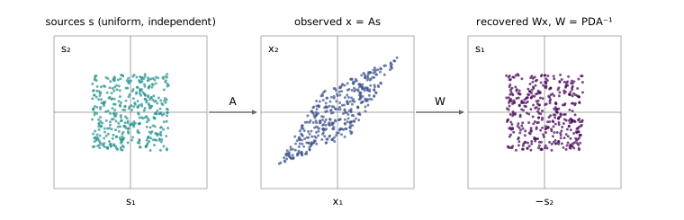
1:15:44 Recovery has unavoidable ambiguities. The first is order. Nothing in the data says which source is the person and which is the radio, so the sources come back in an arbitrary order. The second is sign. A square flipped horizontally or vertically is the same square, so a source can come back negated. For audio that is harmless, because sounds identical to . The official notes add a third, scale. Multiplying a source by and the corresponding column of by leaves unchanged, so the sources are determined only up to scale, and for audio that is only a volume. All three combine into with a permutation and diagonal, as in the right panel of Figure 15.4. The generator checks that every such , including swaps, sign flips and rescalings by 2 and , returns exactly the sources, permuted and rescaled.
The picture also shows what ICA depends on. A uniform square has corners, which mark the original axes. Lecture 16 shows that Gaussian sources, whose density is round, have no such corners, and that this ambiguity cannot be resolved. It then derives the algorithm that finds by maximum likelihood.
PCA, with the variance derivation and the eigenvector solution, is cs229-notes10. The ICA model, its permutation, scaling and sign ambiguities, and the reason Gaussian sources cannot be separated are in cs229-notes11, section 1. The density of a linear transformation and the maximum-likelihood algorithm for are in sections 2 and 3.