19 Finite-Horizon MDPs and the Linear Quadratic Regulator
Lecture 19
finite-horizon MDPs, linear quadratic regulator, LQR, Riccati equation, linearization
Lecture video: Lecture 19: Reward Model and Linear Dynamical System · 1:21:07
Based on the lecture by Andrew Ng — CS229, Stanford University, Autumn 2018.
Fitted value iteration (Section 18.4) handles continuous states by approximating the value function. This lecture finds the one important case where no approximation is needed: if the dynamics are linear and the reward quadratic, the value function is exactly quadratic, the optimal policy is exactly linear, and both come out of a short matrix recursion however many state variables there are. Getting there takes two small generalizations of the MDP first, rewards that depend on the action and a finite horizon, because the algorithm, the linear quadratic regulator (LQR), is most naturally a backward pass over a fixed number of time steps. Ng’s summary is that LQR applies to a narrow set of problems, but when it applies it is the algorithm to use.
19.1 Rewards that depend on the action
4:16 So far the reward has been a function of the state alone. Letting it depend on the action too, , makes the payoff
and it lets a problem say that actions have costs. A robot in a maze can be charged for moving and nothing for standing still. A helicopter can be charged for yanking the sticks hard, which makes it jerk around. A route planner can charge each road segment its own cost, and a factory can price sending a maintenance crew differently from doing nothing. 5:55 Bellman’s equation changes in one visible way:
with the max now outside the immediate reward, since that reward depends on the action being chosen. A student checks that the max covers the whole bracket, and it does. Value iteration uses Equation 19.1 as its update unchanged, and the optimal policy is the argmax of the same bracket. The reward depends on the current state and action, not on the next state. Ng notes that other formulations exist and this is one convenient one.
19.2 Finite horizons and policies that watch the clock
11:00 The second generalization replaces the discount factor with a horizon . The MDP runs for steps and then stops, and the payoff is the finite sum
usually without discounting, though discounting is still allowed. Ng’s example is a model helicopter with thirty minutes of fuel: the aim is to collect as much reward as possible before the clock runs out.
13:11 A finite horizon has a consequence that is easy to miss. The best action can depend on the time. Put a robot between a small nearby and a large farther off. With plenty of time it should go for the . With two or three steps left it should grab the , because the is out of reach. So the optimal policy is written , and is called non-stationary. 15:46 Ng points out what was implicit until now: in the infinite-horizon discounted setting of lectures 16 and 17 the optimal policy is stationary, the same at every step, because the future always looks the same.
16:31 Once the policy may change over time, so may the world. A non-stationary MDP has and indexed by time. Ng gives three examples. A long-haul airliner can burn a third of its take-off weight in fuel, so it handles differently on landing. A drive to San Francisco at 5 pm runs into rush hour, and into mud if the forecast says rain. And in a factory running round the clock, labour costs and availability change with the shift.
19.3 Solving it backwards
21:11 Define as the best expected payoff from state at time to the end. With nothing left after the last step, the base case is just the best immediate reward,
23:27 and each earlier step looks one step ahead to the next:
This is no longer value iteration in the sense of repeating an update until it converges. It is dynamic programming: compute , then from it, then , down to , once each, and read off at every step. Time-varying and slot into Equation 19.2 at no extra cost.
28:31 A student asks whether letting recovers ordinary value iteration. The two are closely related, but undiscounted sums can grow without bound as grows. That is one reason discounting exists. If , a discounted value is at most in size, and a finite-horizon one at most .
30:30 Ng sketches the / corridor with deterministic moves. With two steps left, the values read like “10, 10, 10, 1, 1, 1, 0, 0, 0”: cells within reach of the , cells only within reach of the , and cells that can reach neither. He suggests building the little simulator to watch the policy change as the clock runs down. Figure 19.1 does that for an eleven-cell corridor of our own, with the in cell 0, the in cell 8, and a state-action reward of for each move, so that it uses both of this lecture’s generalizations. The generator checks the dynamic programme against brute force over every action sequence up to seven steps. Cell 5 shows the non-stationarity in full. With one or two steps left it stays put, since nothing is reachable and moving costs. With three or four it heads right for the . With five or more it heads left for the .
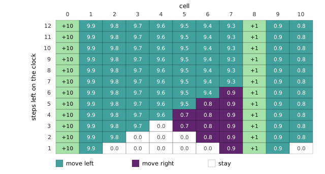
The figure’s caption hides one more lesson. Without discounting and with waiting free, many cells have several optimal actions. Leaving for the now or one step later gives the same total if there is time either way. Discounting is what makes sooner strictly better.
19.4 The LQR model
32:04 LQR is a finite-horizon MDP with continuous states , continuous actions , and two specific assumptions. The first is that the dynamics are linear with Gaussian noise:
with and . 34:27 Ng apologises for the notation. is now both the set of actions and a matrix, because LQR comes from control theory in electrical and mechanical engineering and reinforcement learning from computer science, and when the two literatures met, their letters clashed. The same thing happens to below. 36:30 The second assumption is a quadratic reward,
with and positive semi-definite, so both terms are costs. For a helicopter that should hover at the origin, and give . That penalises drifting from the hover point and penalises large control inputs. Time-varying , , , are allowed but not needed for the derivation.
40:43 Where do and come from? The first way was lecture 18’s (Equation 18.1): fly the helicopter, log trajectories, and fit and by least squares. Ng says again that this gives a good model for slow flight.
19.5 Linearizing a nonlinear model
43:02 The second way starts from a nonlinear simulator , from a physics engine or “a friend with a physics degree”. Ng tried the inverted pendulum’s equations himself and found them complicated. To make it linear, he draws the one-dimensional case. 45:31 Plot against , pick a point , and replace with its tangent line there:
49:05 The tangent is good near and poor far away, so should be where the system spends its time: the hover point for a helicopter, the upright pole at rest for the pendulum. 50:37 With an action as well, linearize around a typical pair using the Jacobians:
53:20 This is affine rather than linear, because of the constant terms. Ng’s fix is to add an intercept to the state, a component fixed at 1. Then Equation 19.5 takes the form after “some algebraic munging”. When the linearization point is the origin and the system rests there, , as for the upright pendulum, the constants vanish and no intercept is needed.
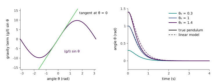
Figure 19.2 does this for a pendulum on a motorised pivot, with the angle measured from upright and a torque as the action. The only nonlinear term is gravity, , and linearizing at replaces it with . The generator checks the hand-derived and against finite differences. The line is 1% too strong at 0.25 rad, 4% at 0.5 rad, 19% at 1 rad and 50% at 1.5 rad. The right panel runs the LQR controller designed on the linear model on the true pendulum. From 0.3 rad the real and predicted trajectories coincide. From 1.4 rad they come apart by up to 0.11 rad, but the controller still brings the pole up. Feedback forgives a model that is wrong in the right direction. Because the measured state is fed back every step, the controller corrects its own model errors as they appear. In this toy, with unlimited torque, it recovers even from 3 rad. A real motor’s torque limit would end that long before.
19.6 The value function is exactly quadratic
56:05 Now run the backward recursion Equation 19.2 on the LQR model. With continuous states, the sum over becomes an expectation over . 57:07 The base case is immediate:
because , so the best last action is . A student notices that is also non-negative. It is, but it cannot be chosen: only is maximised over.
59:09 The inductive step carries the whole method. Suppose
for some matrix and scalar . This holds at with and . 1:04:23 Then
The expectation of a quadratic under a Gaussian is a quadratic of the mean plus a constant, . So the bracket is a quadratic function of , and since and it is concave. 1:06:57 Setting its derivative to zero gives
1:08:03 Ng stops on this. The optimal action is a linear function of the state. He stresses that this is not a function-approximation claim. Nobody fitted a line to the optimal action. Of all functions of the state, linear or not, the best one turns out to be linear. Substituting back into the bracket gives another quadratic in , which completes the induction. 1:09:45 The coefficients obey the discrete Riccati equations:
1:11:04 The whole algorithm is to set and , then apply Equation 19.7 and Equation 19.6 for down to , and finally act with . 1:14:08 What impresses Ng is that nothing in it is approximate. The approximation happens once, when a real system is forced into the form of a linear model with a quadratic cost, by regression or by linearization. After that, the value function really is quadratic and the policy really is linear, and the recursion computes both exactly.
The generator tests each claim by a second route on a cart with position and velocity at 10 Hz and a 60-step horizon. At 20 random times and states, a numerical maximisation of the Bellman bracket lands on and on to within . None of 400 perturbed policies beats , and half of them add nonlinear terms of the state and time.
cs229-notes13 prints the optimal action without the leading minus sign in Equation 19.6. It also prints , and the board in the lecture shows the same minus sign. Both are wrong, and the notes’ own footnote, , gives the plus sign. The noise should make the value worse, and since , only does that. Monte Carlo settles it. From with , 4,000 rollouts of the cart under average . Equation 19.7 predicts , and the printed sign predicts , a positive value for a problem whose rewards are all negative. The action’s sign matters even more. Without the minus, the controller pushes the cart away from the origin, and the payoff of a single noiseless run is . The notes also write where is meant, and and for the same matrix.
Finite-horizon MDPs, LQR and linearization are cs229-notes13, sections 1, 2 and 3.1. Section 3.2 goes on to differential dynamic programming, which re-linearizes around a trajectory instead of a single point. Section 4 covers LQG, LQR when the state is observed only through noise, with the Kalman filter. The lecture covers neither.
19.7 The noise does not change the policy
1:15:22 Ng ends with a property he calls fun, and warns against generalizing. Look at what each quantity depends on. in Equation 19.6 needs but not , which makes sense: adding a constant to every future value cannot change which action is best. in Equation 19.7 needs only . 1:17:36 The noise covariance appears in exactly one place, the update for . Delete the line from the code and the optimal policy is computed perfectly without ever being used. The optimal LQR policy does not depend on the noise. The value does: a helicopter in a gale does worse than one in still air. But the best response to any state is the same in both.
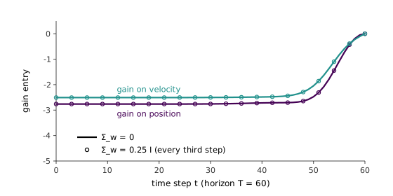
Figure 19.3 shows both effects on the cart. The gains computed with and with are identical to the last bit, while goes from 0 to . The figure also shows the finite horizon at work. For the first half of the horizon the gain is flat at , a stationary policy in all but name. Over the last 25 or so steps it relaxes to zero, because there is less and less future in which a correction would pay off. That is the clock-watching of Figure 19.1 in continuous form.
1:19:00 Ng draws two lessons. The narrow one is that, when applying LQR, there is no need to work hard at estimating . The broader one is about practice. For most MDPs the noise does change the policy, and the form of the noise matters. But in his experience of building robots, remembering to add noise matters more than getting its size exactly right. Ten per cent more or less rarely matters; a factor of two often does. That is the same advice as lecture 18’s (Section 18.3), now with one case where it can be proved.