3 Locally Weighted and Logistic Regression
Lecture 3
locally weighted regression, logistic regression, maximum likelihood, Newton’s method, sigmoid function
Lecture video: Lecture 3: Locally Weighted and Logistic Regression · 1:19:34
Based on the lecture by Andrew Ng — CS229, Stanford University, Autumn 2018.
This lecture takes the linear regression of lecture 2 in three directions. Locally weighted regression keeps the least-squares machinery but refits it around every query point, which lets a straight-line method trace a curve no single set of features would fit. A probabilistic reading of linear regression then shows that least squares is not an arbitrary choice: it is what maximum likelihood gives when the noise is Gaussian. And the same two-step recipe — assume a distribution for given , then maximise the likelihood — produces logistic regression, the first classification algorithm of the course, along with Newton’s method to fit it in a handful of iterations. Ng ranks linear and logistic regression as the two learning algorithms he uses most.
3.1 Features, or a different algorithm
2:20 Lecture 2 fitted a straight line to house prices, but the data may bend. One answer is to change the features: fit by defining , and the linear-regression machinery runs unchanged, because “linear” refers to the parameters, not to . The trouble is choosing. A quadratic eventually curves back down, which for house prices says a bigger house is cheaper; or might bend the right way; and for data that rise, dip and rise again, Ng says frankly that finding the right set of features — square root, log, cube, — is hard. Feature-selection algorithms that automate the choice come later in the course.
5:53 Locally weighted regression sidesteps the question, and it introduces a distinction worth having early. A parametric learning algorithm fits a fixed set of parameters, after which the training set can be erased: linear regression keeps only . A non-parametric algorithm has to keep the data, and the amount it stores grows — linearly here — with the size of the training set. That is the cost of not having to choose features, and it is why Ng warns that such methods may not suit a really massive dataset.
3.2 Locally weighted regression
8:33 Linear regression makes a prediction at by fitting once to all the data and returning . Locally weighted regression postpones the fit until it knows where the prediction is wanted. Given the query point , it fits a straight line that pays most attention to the training examples with inputs near , glances at the ones further away, and uses that local line to predict at ; a different query point gets a different line. Formally it chooses to minimise a weighted cost,
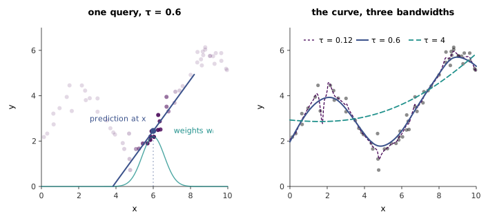
and returns . 12:09 When is close to the query the weight is near and that example’s error counts in full; when it is far the weight is near zero and its error term all but disappears from the sum. (Ng first wrote the exponent without the square on ; a student caught it, and it is .) The left panel of Figure 3.1 shows one such fit.
figures/03-locally-weighted-logistic/make_diagrams.py.
15:27 The weight function is shaped like a Gaussian bell, and Ng heads off the obvious confusion: it has nothing to do with a Gaussian density. Its peak is 1, it does not integrate to 1, and it is not a probability of anything — just a convenient bump. The bump’s width is the bandwidth , a hyperparameter, and 16:46 it decides how large a neighbourhood each local fit sees. Ng leaves its effect for the problem set, saying only that it controls overfitting and underfitting; the right panel of Figure 3.1 shows both. With only a couple of points carry weight in each fit, and the curve chases the noise into spikes; with nearly every point carries weight everywhere, and the curve flattens towards a single straight line. In the limit it is that line: the generator checks that a bandwidth of reproduces the ordinary least-squares fit to four decimal places. At the curve follows the rise, the dip and the plateau without being told what features describe them.
The questions that followed are the practical ones. Asked 18:53 about predicting outside the range of the data, Ng said the formulas still work but the results may be poor — locally weighted regression is not good at extrapolation, but then most learning algorithms are not. Asked about letting vary across the input space, he said yes: there is a large literature on choosing it from the local density of points, and on replacing the bell with other shapes, such as a triangle that reaches zero outside a window. His own rule 19:58 is to reach for locally weighted regression when the number of features is small, two or three, there is a lot of data, and you do not want to think about which features to use.
20:29 On cost, his answer at the board needs one correction. Each prediction solves a weighted version of the normal equations, with the diagonal matrix of weights, and that is a system of dimension — the number of parameters — not of the number of training examples, as the lecture puts it. What does grow with is the work of forming the system, since every training example contributes a weighted term, and that work is repeated for every query. So a prediction costs time proportional to , which is why a few thousand examples are no problem and millions call for data structures such as k-d trees that find the nearby points without visiting all of them.
Locally weighted linear regression, with the same weight function, is cs229-notes1, section 4; the problem set explores the bandwidth.
3.3 Least squares as maximum likelihood
22:24 Lecture 2 promised a reason for squaring the error. Ng’s answer starts by assuming how the data were generated: each house’s price is a linear function of its features plus an error,
where gathers everything the model leaves out — the seller’s mood that day, unmodelled features — and random noise. The density of the error is the Gaussian , which, unlike the bump of Section 3.2, does integrate to one. 25:45 The large assumption is that the errors are IID — independent and identically distributed across houses — and Ng is candid that it is false: if one house on a street is priced unusually high, its neighbours probably are too. It is one of those assumptions that is probably not true and is good enough to give a useful model.
Together the assumptions say that, given and , the price is Gaussian around the line:
28:16 The semicolon is read “parameterised by”. Writing a comma would mean conditioning on , which is not a random variable in this frequentist view; Ng keeps the distinction, he says, mostly to avoid upsetting statistician friends, and admits it changes nothing about the code one writes.
30:57 Because the errors are independent, the probability of all the observed prices is the product of the individual densities, and viewed as a function of with the data fixed that product is the likelihood,
32:44 Ng’s vocabulary rule is worth adopting. The likelihood of the parameters and the probability of the data are the same number; which name you use says which argument you are varying. So one speaks of the likelihood of the parameters and the probability of the data, never the reverse.
37:49 Maximum likelihood estimation chooses the that makes the observed data most probable. The logarithm is strictly increasing, so it is easier and equivalent to maximise the log-likelihood , which turns the product into a sum:
The first term does not involve , and is a positive constant, so maximising is exactly minimising the least-squares cost of lecture 2 — and the answer does not depend on at all. Least squares is maximum likelihood under IID Gaussian noise.
Asked 35:31 why the noise should be Gaussian, Ng pointed to the central limit theorem: an error made of many small, not-too-correlated contributions — the seller’s mood, the school district, the weather, transport — sums to something close to Gaussian, which is why it became the default. The same derivation also answers lecture 2’s question about absolute error, which Ng deferred. Assume instead that the errors follow a Laplace distribution, with density proportional to , and the log-likelihood becomes a constant minus a multiple of : maximum likelihood is then least absolute deviations. The difference is not cosmetic. With an intercept alone the Gaussian answer is the mean and the Laplace answer is the median, and the generator checks both against a grid search on a sample of twenty values around 3 plus one at 25: the Gaussian estimate is pulled to 4.09 by the single outlier, the Laplace one stays at 2.93. The choice of noise model is a choice of how much to trust the extreme points.
Asked 41:07 whether some other cost would ever be better, Ng said that under these assumptions none is — the derivation makes least squares the answer. If you know the errors are badly non-IID, more sophisticated models exist, but in practice he rarely bothers: assumptions known to be not quite true are often kept because they make the algorithm efficient.
The same derivation is cs229-notes1, section 3, which also notes that the conclusion does not depend on .
3.4 Why not linear regression for classification
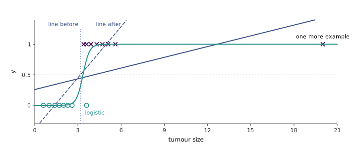
43:42 The recipe — assume , then maximise the likelihood — now goes to a problem where is 0 or 1: binary classification, with lecture 1’s tumours as the example. The tempting shortcut is to fit a straight line to the 0/1 labels and call anything above 0.5 a 1. Ng’s objection 44:43 is a single extra example. Add one malignant tumour far to the right, a point whose label nobody would dispute, and the least-squares line tilts to reach it; the place it crosses 0.5 slides right, and malignant tumours that were correctly classified are now called benign. In Figure 3.2 the threshold moves from 3.17 to 4.11, and the number of misclassified tumours goes from one to three, because of a point that contained no new information about where the boundary is. There is also the unnatural fact that a line outputs values below 0 and above 1 for something that can only be 0 or 1. Ng says some people use linear regression for classification and sometimes get lucky; he never does.
figures/03-locally-weighted-logistic/make_diagrams.py.
3.5 The logistic model
46:46 A classifier’s hypothesis should output a number between 0 and 1, so logistic regression passes the linear function through the sigmoid or logistic function — the two names mean the same thing:
starts near 0 for very negative , passes through at and approaches 1. Ng is open that he is pulling it “out of a hat” for now: many functions have that shape, and lecture 4 derives this one from the generalised linear model framework. Section 3.6 adds a reason of its own.
50:23 The probabilistic assumption is that the hypothesis is the probability of the positive class — the chance that the tumour is malignant:
A student asked whether the roles could be swapped; they could, and nothing would change except which class is called positive. 52:46 Since is 0 or 1, the two lines compress into one,
because whichever factor carries a zero exponent becomes 1 and drops out, leaving the line that applies. The trick is only notation, but it is what makes the likelihood a single product.
3.6 Maximum likelihood and gradient ascent
56:03 With Equation 3.8 the likelihood is , and its log is
To fit, 58:54 Ng uses batch gradient ascent: the same walk as lecture 2, but uphill, since the goal is now to maximise rather than minimise , so the minus sign in the update becomes a plus. Working out the derivative, which Ng leaves to the notes, gives
The generator checks this gradient against finite differences of Equation 3.9.
1:03:06 Ng then put a question to the room. Flip the sign and swap the two terms in the bracket, and Equation 3.10 is character for character the LMS rule of lecture 2 — yet the lecture had just argued that linear regression is wrong for classification. What changed? The hypothesis: is now , not , so the same-looking update does something different. The resemblance is not a coincidence; it holds for the whole family of generalised linear models, and Ng adds that the likeness caused priority disputes in the field’s early history, between people who thought the algorithms were one and people who saw they were not.
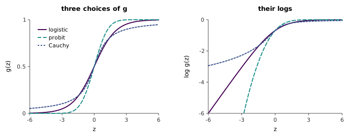
1:02:15 Asked whether has local maxima, Ng said no: for logistic regression the log-likelihood is concave, so the only maximum is the global one. The Hessian makes that checkable, , a negative sum of outer products, and the generator confirms it is negative semidefinite at two hundred random parameter values. He then gave this as another reason to choose the logistic function over other S-shaped functions — that it guarantees a single maximum. That is true but not unique to it, and the generator says where the property actually comes from. is concave because and are both concave in , and that is a property of the S-curve, not of logistic regression. The normal CDF, which gives probit regression, has it too. The Cauchy CDF, , an S-curve with heavy tails, does not: its log bends upward in the left tail (Figure 3.3), and on a three-example dataset the resulting log-likelihood has positive curvature at , so the argument that rules out local maxima no longer applies. The logistic function is one of a class of choices with a single maximum, not the only one; its claim to being the choice is the generalised-linear-model derivation of lecture 4.
figures/03-locally-weighted-logistic/make_diagrams.py.
Asked 1:04:53 whether logistic regression has an equivalent of the normal equations, Ng’s short answer was no: there is no known closed form for the maximising , so an iterative method is always needed.
The derivative of the sigmoid, , and the derivation of Equation 3.10 from it are in cs229-notes1, section 5.
3.7 Newton’s method
1:05:36 Gradient ascent takes baby steps. Ng’s comparison is a problem that needs a hundred or a thousand gradient iterations and only ten of Newton’s method, each of which costs more. To explain it he solves a different problem first: given a function of a single real , find where . Maximising is such a problem, since at the maximum , so in the end will be .
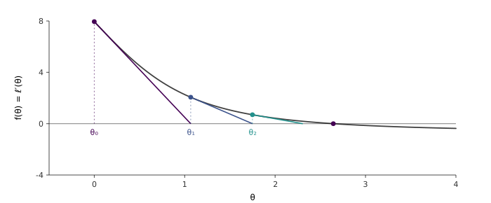
1:08:33 The picture is a sequence of tangents. From the current guess, draw the line tangent to and follow it down to where it crosses zero; that crossing is the next guess. Repeat, and within a few iterations the guesses sit on the root (Figure 3.4). If the tangent at meets the axis a horizontal distance away, its slope is the height over the run, , so and
figures/03-locally-weighted-logistic/make_diagrams.py.
The update uses only where vanishes, so it is the same whether the goal is a maximum or a minimum — the official notes leave this as a question, and that is the answer. What makes it the right tool here is that is concave, so its only stationary point is the maximum.
1:14:22 The speed has a name, quadratic convergence, which Ng calls “not a great name”. Informally, once Newton’s method is close, the error is roughly squared at each step: an error of 0.01 becomes about 0.0001 and then about 0.00000001, so the number of correct digits doubles per iteration. On the problem of Figure 3.4 the generator’s errors run 0.053, then 0.0014, then . The doubling only starts near the root; from the start at zero the first few steps shrink the error more slowly.
1:16:03 With a vector, the first derivative becomes the gradient and the second the Hessian , the matrix of second partial derivatives :
1:17:22 That matrix is the catch. Each iteration solves a linear system in it, or inverts it, which is nothing for ten parameters and prohibitive for a hundred thousand. Ng’s rule of thumb follows: with ten or fifty parameters he would very likely use Newton’s method and be done in a few iterations; with ten thousand or more he would use gradient descent. The gap in iteration counts can be far larger than his hundred-to-ten. On the tumour data of Figure 3.2, which are nearly separable and so put the maximum far out at , Newton’s method reaches it to six decimal places in 9 iterations; gradient ascent with the safe fixed step needs about 117,000.
Newton’s method and its vector form are cs229-notes1, section 7, which adds that Newton’s method applied to the logistic log-likelihood is also called Fisher scoring.