18 Robot Learning
Lecture 17
Based on Lecture 17 of CS231n, Stanford University, Spring 2025, given by Yunzhu Li.
18.1 Closing the loop
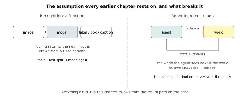
Every model in this book so far has been a function. An image goes in, a label or a box or a mask or a sentence comes out, and the transaction ends there: nothing the model produces affects what it will be shown next. That property is so deeply assumed that it is rarely stated. It is what licenses splitting a dataset into train and test, what makes the samples independent enough for the loss to be a sum over them, and what lets a benchmark number mean anything at all.
A robot breaks it. The action a robot takes changes the state of the world, and the changed world is the next observation. The data the robot will be trained on tomorrow is a consequence of the policy it is running today, which means the training distribution is not a fixed thing to be sampled but a moving object the learner itself is dragging around. Almost everything difficult in this chapter follows from that one fact, and it is worth holding on to as the organising idea rather than as a caveat.
The framework that replaces the function has four parts, and the whole field is phrased in them. At each time step the agent observes a state , chooses an action , and the environment responds with a new state and a scalar reward measuring how well things are going. A policy is what maps states to actions, and the objective is not to be right about any single step but to maximise the reward accumulated over a whole episode:
where discounts rewards that arrive later, and the expectation is over whatever randomness the environment and the policy contain. The discount is not only a modelling convenience; it is what keeps the sum finite when the episode has no natural end.
The formulation is worth taking seriously partly because of how far it stretches. Balancing a pole on a cart makes the state the pole’s angle and angular velocity together with the cart’s position and speed, the action a horizontal force, and the reward one unit for every step the pole stays upright. Legged locomotion makes the state the angles and velocities of every joint, the action a torque per joint, and the reward one unit per step taken while still standing. Playing Atari makes the state the raw screen and the action a joystick direction, with the reward the change in score. Go makes the state the board, the action where to place the next stone, and the reward a single bit delivered at the end of the game. Even a language model fits: the state is the text so far, the action is the next token, and a chatbot optimised against human preference is an agent whose reward is a person’s satisfaction with the reply.
That range is the formulation’s strength and also the source of a mistake worth heading off early. The fact that Go and cloth folding can be written down the same way does not make them the same problem, and the difference is not merely one of difficulty. In Go the state is exactly and completely observable, the transition function is known perfectly, and the reward is unambiguous. In cloth folding none of the three holds. The state is whatever a few cameras can see of a self-occluding deformable object; the transition function is the physics of fabric, which nobody can write down at the resolution needed; and the reward is a human judgement about whether the result looks folded. Three different people will fold a shirt three different ways, and each will be satisfied with the outcome. There is no unique goal state to reach and therefore no unique reward function to optimise, only a family of them corresponding to what different users happen to want — smallest folded area, fewest creases, fastest completion. The reward is a design decision, and pretending otherwise is how a well-optimised policy ends up doing something nobody asked for.
So the honest way to state the difference from the rest of the course is this. Computer vision, in the form the previous chapters treat it, is a representation-learning problem: given high-dimensional input, produce a useful description of it. Robot learning is a constrained optimisation problem in which the constraints are physics, the objective is defined over a goal, and the variable being solved for is a sequence of actions. The perception is still there, and it is still hard, but it has stopped being the answer and become a component inside a loop.
18.2 What makes robot perception a different problem
The last chapter ended by observing that its models represent the compositional structure of a scene least well, and predicting that this is exactly what a robot cannot do without. This section is where that prediction starts to be paid, and the reason is that a robot needs a different kind of answer than a caption or a mask.
Consider what Section 17.8 established. Molmo’s contribution was to make pointing a first-class output: the model emits 2D coordinates rather than text, and the same coordinate grounds a referring expression, enumerates instances for counting, and — the part that matters here — hands a target to something downstream. A point is a navigation waypoint or a grasp target. That is already an action interface, and it is the cleanest bridge between the two chapters: it is the moment a vision model stopped producing a description of the world and started producing something a controller can consume.
But a point is only the beginning of what a manipulation policy needs, and the gap between them is the substance of robot perception. A grasp needs the object’s 3D pose, not its image coordinates. A push needs to know how the object will move when pushed, which depends on its mass distribution and its friction against the table. Folding a shirt needs the configuration of a surface that is mostly hidden behind itself. None of those are recoverable from a single labelled frame, and all of them are compositional in the strict sense: they are facts about parts and their relations, not about the identity of a whole.
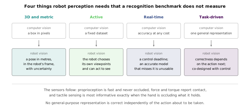
Four differences separate this from computer vision as the course has treated it, and it is worth being precise about each because each one closes off a technique that worked earlier.
The first is that robot vision is 3D and metric. A detector that reports a bounding box in pixels has said nothing a gripper can use; the robot needs a pose in metres, in its own coordinate frame, with an uncertainty attached. This is why depth is not an optional extra channel in robotics the way it often is in vision benchmarks, and it is why the geometry of Section 16.1 is closer to the working practice of robotics than object detection is.
The second is that the robot is an active perceiver. A vision dataset is a fixed collection of images somebody else chose; a robot chooses its own viewpoints and can act in order to see. If an object is occluded, the robot can move the camera, or move the occluder, or rotate the object in its hand — and these are the same kind of decision as the manipulation itself, made by the same policy against the same objective. Perception stops being a preprocessing stage and becomes one of the things the policy is for.
The third is that it is real-time and closed-loop. A model that takes two seconds per frame is unusable for a controller that must issue commands at tens of hertz, no matter how accurate it is. This constraint is unfamiliar from the rest of the course, where latency appears as an engineering footnote, and it is severe enough to be an architectural constraint: it is why the models of Section 18.7 are measured in control frequency as much as in success rate, and why a 35-million-parameter policy running at 3 Hz was a headline result rather than an embarrassment.
The fourth is that it is task-driven, and this is the one that most changes what “good perception” means. There is no general-purpose representation that is correct independently of what the robot is about to do. Segmenting every object in the scene to pixel accuracy is wasted computation if the task is to push one pile of coffee beans into a square, and a representation that captures the beans as a coarse distribution is better in the strict sense of leading to better actions. Perception and control are co-designed, and the criterion for a representation is whether a policy or a planner built on it works — not whether it scores well on a perception benchmark.
The sensor suite reflects all four. Cameras and depth sensors supply the scene, but proprioception — the joint encoders reporting the robot’s own configuration — is the signal a controller most depends on, because it is fast, accurate, and never occluded. Force and torque sensing at the wrist reports contact, which vision cannot see at all: whether the gripper is actually holding something, and how hard. Tactile sensors in the fingers report whether a grasp is slipping. These are complementary in an important way, since the moments when vision is least informative — when the hand is on the object, occluding it — are exactly the moments when contact sensing is most informative.
18.3 Four things the reward has to pay for
Reinforcement learning is the most direct response to Equation 18.1: let the agent act, observe what reward comes back, and shift its behaviour towards whatever produced more of it. Nothing supervises the individual action. The only signal is a scalar arriving from the environment, and everything the agent knows about which of its thousands of decisions were good has to be extracted from that scalar. Four properties separate this from the supervised loop of the earlier chapters, and each one is a place where a technique that worked there stops working.
The first is that the environment is stochastic, so the same action twice does not produce the same outcome. Push a box across a table and the distribution of contact forces under it — which no sensor reports — decides whether it slides straight or rotates, and by how much. The consequence is that reward is a random variable rather than a measurement, and a single trajectory is a single sample from it. An action that was correct can be followed by a poor reward and an action that was wrong by a good one, so the learner cannot trust any individual outcome and has to average over many.
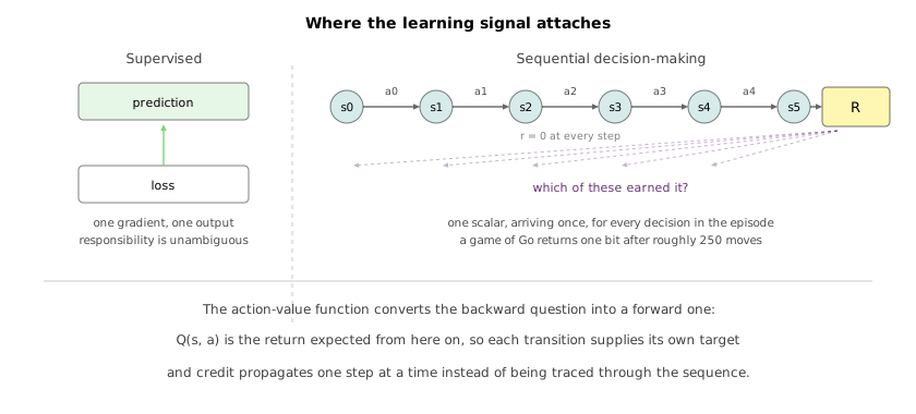
The second is credit assignment, and it is the one the field has spent the most effort on. In supervised learning the loss attaches to the prediction that caused it: the gradient of a cross-entropy against a label points at the specific output that was wrong. In sequential decision-making the reward is delayed, sometimes until the very end. A game of Go returns one bit after roughly two hundred and fifty moves, and the move that lost the game may have been the fortieth. The learner must distribute a single scalar over a long sequence of decisions with nothing telling it which of them deserved it.
The third is that the environment is not differentiable. The supervised chain from input through model to loss is differentiable end to end, which is what makes backpropagation applicable at all. The chain from action to reward passes through physics, or through a game engine, or through a human’s judgement, and none of those admits a derivative. So the gradient of reward with respect to action has to be estimated by sampling — by trying variations and inferring a direction from the differences in return. Zeroth-order estimates like this have variance that grows with the dimension of the action space, which is the technical root of why reinforcement learning needs so much data. It is not that the algorithms are wasteful; it is that a sampled gradient carries far less information per interaction than a computed one.
The fourth is non-stationarity, and it is the closing of the loop from Section 18.1 restated in the language of training. In supervised learning a prediction does not affect which example comes next, so the data distribution is fixed and the i.i.d. assumption holds. Here the states the agent visits are generated by the policy the agent is currently running, so improving the policy changes the distribution the policy is being evaluated on. The target moves because the learner moved it.
The classical answer to credit assignment is to learn a function that answers the counterfactual directly. The action-value function is the discounted return expected from taking action in state and following afterwards:
If this function were known for the optimal policy, acting would be trivial: evaluate for every available action and take the largest. That is the whole of the decision rule, and it is why is worth the trouble. What makes it learnable without waiting for episodes to finish is that it satisfies a consistency condition relating each state to its successor,
so a single observed transition gives a target for built out of evaluated one step later. Learning becomes regression of the network against its own slightly-more-informed estimate, and the reward propagates backwards along the trajectory one transition at a time. Credit assignment is solved not by tracing responsibility through the sequence but by defining a quantity whose value at each step already contains the future.
Deep Q-learning made this work on raw pixels, and the architectural detail that matters is small and easily missed. Rather than taking a state and an action and returning one number — which would need a separate forward pass per action — the network takes only the state, four stacked frames of the Atari screen so that velocity is recoverable from a static input, passes them through convolutional layers and a fully connected head, and emits one value per action in a single pass. Choosing an action is then an over the output vector. The same network, the same hyperparameters and no game-specific features were applied to seven Atari 2600 games, and the result outperformed all previous methods on six of them after ten million frames.
What that trained agent does is the best argument for the whole approach. On Breakout, ten minutes of training produces a paddle that occasionally touches the ball. Two hours produces one that reliably returns it. Several hours produce something nobody wrote down: the agent learns to dig a tunnel up the side of the brick wall and send the ball behind it, where it bounces along the top clearing rows without further intervention. That strategy was not demonstrated, not rewarded specially, and not anticipated. It is what exploration under a scalar objective can find when the objective is the only thing specified, and it is the reason the framework is worth its costs.
18.4 Where scale worked, and what it cost
Go is the canonical demonstration, and the sequence after it is instructive because each step removed something rather than adding it. AlphaGo beat a professional player in January 2016 using a policy network bootstrapped from human games, a value network, and Monte Carlo tree search. AlphaGo Zero removed the human games — it learned from self-play alone — and was stronger. AlphaZero removed the Go-specific parts and applied the same algorithm to chess and shogi. MuZero removed the rules of the game, learning a latent dynamics model good enough to plan in without ever being told how the environment transitions — which is the first appearance in this chapter of the idea Section 18.5 is built on.
The lesson usually drawn from that sequence is Sutton’s bitter lesson: the methods that win in the long run are the ones simple enough to absorb more computation, and hand-engineered structure tends to be a ceiling rather than a floor. It is a fair reading of the games results, and it is worth stating precisely because the rest of this chapter is largely about the conditions under which it does not transfer. In November 2019 Lee Sedol retired from professional Go, saying that an entity that cannot be defeated had appeared. Between then and now the same recipe, scaled further, produced strong agents for StarCraft II and Dota 2, games with vastly larger state spaces than Go. The empirical claim is close to unconditional: given a well-specified game and sufficient compute, reinforcement learning will produce a superhuman player.
The phrase carrying all the weight is well-specified game. A game has a perfect simulator — the rules — that runs faster than real time, resets instantly, never wears out, and is exactly the environment the agent will be evaluated in. Every one of those properties fails for a robot, and what happens when they fail is best seen in the two robotics results the lecture uses.
The first is legged locomotion. ANYmal trained by Lee and colleagues walks over terrain that defeated previous controllers — loose rubble, mud, snow, running water — using only proprioception, with no vision at all. The interesting part is the training structure, which exists precisely because the simulator and reality diverge. Training a rough-terrain controller directly from the sensors the real robot has is too slow to converge, so the work splits it in two: a teacher policy is trained in simulation with access to privileged information the real robot could never have — the exact terrain profile, the ground-truth contact state of each foot — and then a student policy that sees only the proprioceptive history available on hardware is trained to imitate the teacher. The privileged information makes the problem easy enough to solve; the imitation step converts the solution into one that can actually be run. The student has to infer from the history of joint positions and torques what the teacher was told directly, and it does, recovering contact and slip events from proprioception alone.
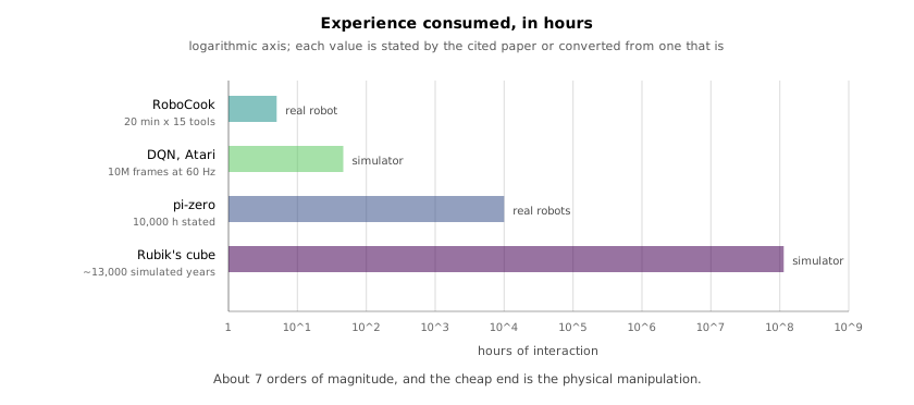
The second is dexterous manipulation, and it is the honest one. OpenAI trained a five-fingered hand to manipulate a Rubik’s cube, using automatic domain randomisation — a distribution over simulated physics whose difficulty is increased whenever the policy is doing well, so the policy is forced to become robust to a range of dynamics wide enough to contain reality. The result is genuinely impressive and the accounting is sobering. The policy consumed roughly thirteen thousand years of simulated experience, trained on 64 V100 GPUs alongside 29,440 CPU cores for rendering and simulation, continuously for several months. And it does not reliably solve the cube: on a fixed fair scramble repeated ten times, it completed a sequence requiring fifteen face rotations 60 % of the time, and the full twenty-six-rotation scramble 20 % of the time. A more recent controller for in-hand reorientation of novel shapes reorients objects it never trained on with a median time near seven seconds, and drops a duck-shaped test object in 56 % of trials.
Three bottlenecks explain the gap between the games results and these, and they are the reasons the rest of the chapter exists.
Sample cost. The number of interactions model-free reinforcement learning needs is enormous — Figure 18.4 puts it against the alternatives — and it is not an implementation defect but a consequence of the zeroth-order gradient described above. In a simulator that cost is a compute bill. On hardware it is impossible: thirteen thousand years does not fit in a laboratory, and a real robot executing millions of trials wears out its own actuators long before convergence.
Reward design. A game hands you the reward. A manipulation task does not, and writing one is a design problem with no correct answer, as Section 18.1’s folded shirt already showed. Worse, the optimiser is adversarial towards any specification that is even slightly wrong: reward the robot for lifting the object and it will learn to nudge the object up and drop it repeatedly, because that is what the reward literally asked for. Every practical result above rests on a reward function that took considerable human effort to shape, which means the human labour was not eliminated but moved.
The simulation-to-reality gap. Training in simulation is what makes the sample cost survivable, and it introduces the problem that the policy is optimal for a physics that is not the one it will be deployed in. Friction, compliance, actuator delay, sensor noise and contact dynamics are all approximations, and contact is the worst of them — precisely the regime manipulation lives in. Domain randomisation is the standard answer, and it works by asking for a policy robust across a family of dynamics wide enough to contain reality. The cost is that robustness is bought with conservatism and with more samples, since the policy must solve many environments rather than one.
18.5 Learning the model instead of the policy
Reinforcement learning discards something on every trial. The agent acts, receives a scalar, and updates a policy — but the transition it just observed, the fact that this push moved that object this far, is thrown away once its contribution to the return has been absorbed. That transition is a far richer piece of information than the reward attached to it, and it is available for free on every interaction.
This is also not how people work. Asked to push a mug towards the edge of a table, nobody tries it a thousand times to find out what happens. They know roughly what will happen, because they carry a predictive model of everyday physics accurate enough to plan against, learned from a lifetime of ordinary interaction rather than from a reward signal. The proposal of this section is to give a robot the same thing: learn a forward model
by ordinary supervised regression on observed transitions, and then get the actions by inverting it. Note what has happened to the learning problem. Fitting is supervised learning with dense targets: every step of every trajectory supplies an input–output pair, whether or not the trajectory succeeded, and there is no credit-assignment problem because the label for each transition is the very next observation. Failure data is as informative as success data. The delayed-scalar difficulty of Section 18.3 has not been solved so much as routed around.
Planning is then the inverse problem. Given the current state and a goal, search for the action sequence whose predicted outcome is closest to the goal:
where is a distance in whatever space the state lives in and is the planning horizon. Because is a neural network, this objective is differentiable in the actions and can be optimised by gradient descent through the unrolled model — or, in practice more often, by sampling thousands of candidate action sequences in parallel on a GPU and keeping the best, which costs no gradients and copes with objectives that are not smooth.
The model will be wrong, and the standard defence is to not trust it very far. Only the first action of the optimised sequence is executed; the true next state is then measured, and the whole optimisation is redone from there. This is model-predictive control, and it converts an open-loop plan into a closed-loop policy: prediction error does not accumulate over the horizon because the horizon is restarted at every step. It is the same receding-horizon idea that reappears, for a quite different reason, in Section 18.6.
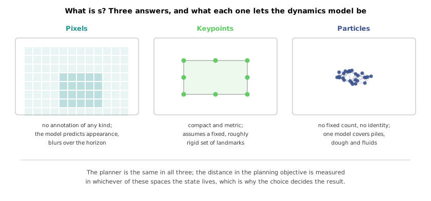
None of that is the hard part. The hard part, and the actual research question, is the one Equation 18.4 quietly assumes an answer to: what is ? A dynamics model is only as good as the state it is a function of, and the history of this area is best read as a sequence of answers to that question.
The first answer was pixels. Deep visual foresight learns an action-conditioned video prediction model — given the current frame and a candidate arm motion, predict the frame that results — and plans by choosing the motion whose predicted frame moves a designated pixel closest to its target. The appeal is that nothing needs annotating. The robot collects its own pushing data autonomously, the supervision is the next frame, and no notion of an object appears anywhere in the system. The cost is that the model has to spend its capacity predicting the appearance of everything in view, including the tabletop and the shadows, when what the plan depends on is the motion of one object. Prediction in pixel space is also blurry over any useful horizon, and blur is precisely the failure mode that destroys a distance metric.
The second answer was keypoints. Keypoints into the future replaces the image with a small set of 3D points, obtained from self-supervised dense correspondence, that track the same physical locations on an object across time. The latent state becomes a few dozen numbers instead of a few hundred thousand, the dynamics model becomes correspondingly easier to fit, and the goal is specified directly as a target configuration of the same keypoints — which makes the distance in Equation 18.5 a distance in metres rather than in pixel intensities. The limitation is in the assumption: a fixed set of keypoints presumes an object with a fixed and roughly rigid structure. A pile of rice has no keypoints.
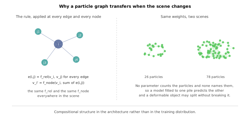
The third answer is particles, and this is where the chapter’s connection to the last one gets paid. Represent the scene as a set of points with no fixed identity, build a graph over them by connecting points that are near enough to interact, and learn the dynamics as message passing on that graph. Each edge computes an interaction from the pair of nodes it joins, and each node updates itself from its own state and the sum of the interactions arriving at it:
Two properties follow from the fact that and are shared across every particle and every pair, and both are the reason this representation works where the previous two do not. The model is indifferent to how many particles there are, so a model trained on one pile of coffee beans transfers to a larger pile without retraining. And it is indifferent to which particle is which, so there is no correspondence to maintain when a deformable object changes shape or a pile splits in two.
This is compositional structure in the strict sense that Section 17.8’s models lacked it. The last chapter closed by observing that a model trained to match captions against random negatives learns which entities are present without learning how they compose, and that the omission would matter here. A particle graph is the opposite arrangement: it represents only entities and their relations, and the physics it predicts is assembled from a local rule applied everywhere rather than recognised as a whole. That is why it generalises across object count, object size and object shape — the composition is in the architecture rather than in the training distribution.
The results follow the representation. Dynamic-resolution particle models manipulate piles of granular material — coffee beans, almonds, candy, granola, rice, corn — gathering them, sorting two mixed kinds, and redistributing a pile into complicated target shapes including letters of the alphabet. The refinement worth naming is that the resolution is not fixed: a regressor predicts how coarse the particle representation should be at each control step, because a task’s early stages need only a rough sense of where the mass is while its final stages need fine detail to match a shape’s boundary. Choosing granularity per step outperforms any fixed choice.
RoboCook is the most complete version of the argument and it makes a dumpling. The robot has four RGB-D cameras reconstructing the workspace into a point cloud, fifteen 3D-printed tools it can pick up and exchange, and a graph dynamics model of the dough learned from real interaction. Producing a dumpling from a lump of dough takes nine stages, and control operates at two levels: a classifier chooses which of the fifteen tools suits the current state and the goal, and a low-level module chooses the motion to execute with it. That low-level module is where the model earns its place — candidate actions and tools are sampled, the graph model predicts the resulting dough shape for each, and the one whose prediction lands closest to the target is selected. Because sampling at test time is slow, the sampling is done offline to generate a dataset and a policy is distilled from it, so the deployed system runs fast while still being derived entirely from the learned model’s predictions.
Two things about that system are worth more than the demonstration. The first is what happens when a person interferes: a human repeatedly deforms the dough while the robot works, and at one point flattens a shape the robot had just cut. The robot does not fail and does not blindly continue. Because the tool classifier is a function of the current observation rather than of a step counter, an observation matching an earlier stage is simply routed back to that stage, and the robot redoes the work. Recovery is a consequence of having framed control as a function of state rather than as a script, which is worth noticing because nothing in the system was designed for disturbance rejection.
The second is a comparison the authors ran and the result is not the expected one. The obvious alternative to learning dough dynamics is to simulate them with a physics engine built for deformable material — the material point method — and identify its parameters from data. They did that, with extensive system identification, and the identified simulator’s predictions were noticeably less accurate than the model learned directly from real interaction. This is worth sitting with, because it inverts the usual framing of the sim-to-real gap from Section 18.4. There, simulation was the cheap source of experience and reality the thing to transfer to. Here, twenty minutes of real interaction per tool produced a better model of this particular dough than a principled simulator fitted to the same data, because the learned model is free to absorb everything the physics engine’s assumptions leave out. Sim-to-real is not a fixed toll to be paid; whether simulation helps depends on how well its assumptions match the material, and for contact-rich deformable manipulation they match poorly.
18.6 Imitation, and two ways it goes wrong
Reinforcement learning learns the policy and pays for it in interactions. Model learning learns the dynamics and pays for it in the difficulty of choosing a state representation. The third option is the one that sounds too simple to work: have a person demonstrate the task, record what they did, and fit a policy to the recording by supervised learning. This is behaviour cloning, and it is a straightforward regression of actions on observations,
over a dataset of demonstrated observation–action pairs. No reward function has to be designed, no exploration is needed, nothing has to be simulated, and the task specification is carried implicitly by the demonstrations. It is by a wide margin the fastest route to a robot that does something in the physical world: collect data in the morning, train overnight, and have a working policy by the following afternoon.
Two things go wrong with it, and they are worth separating because they have different causes and different fixes.
18.6.1 The distribution the policy makes for itself
The first failure is the closed loop of Section 18.1 arriving in its most concrete form. Equation 18.7 is fitted on the states the expert visited, but at deployment the states are the ones the learner visits, and those diverge. A small error moves the robot slightly off the demonstrated trajectory, into a state slightly less well covered by the training data, where the policy is slightly less reliable and makes a larger error, which moves it further off. The training loss can be small and the deployed behaviour still leave the data distribution entirely.
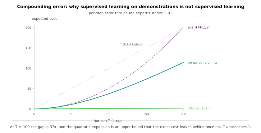
The size of that effect is worth computing rather than gesturing at, because the standard statement of it is imprecise in a way that matters. Take the worst case behind DAgger: a policy that errs with probability per step on the expert’s distribution and, having erred once, stays off the distribution and pays unit cost for the rest of the episode. Its expected total cost over horizon is the probability of having erred by each step, summed:
The generator behind Figure 18.7 evaluates both sides independently and checks that they agree, which is worth doing because the expansion everyone quotes is derived from the left-hand side and loses something on the way. For small the sum is , not : the growth is quadratic, but the leading constant is one half and the is real. And the expansion is an upper bound that the exact cost outgrows its resemblance to — the exact cost can never exceed , since an episode cannot cost more than its own length, so the quadratic regime holds only while is small and after that the curve bends into total failure rather than continuing to accelerate. At and the exact cost is already only 85 % of its quadratic approximation.
The contrast with training on the learner’s own distribution is stark. If the policy is corrected at the states it actually visits, the errors do not compound and the cost is — linear. At and a horizon of 100 steps, that is a cost of 1 against 37, and by 400 steps the ratio is 76.
That is precisely what DAgger does. Train a policy on the demonstrations, run it, and record the states it visits; ask the expert what they would have done at each of those states; add those corrections to the dataset and retrain. The point is not that the expert demonstrates the task better the second time but that they demonstrate it somewhere else — on the states the learner’s own mistakes produce, which is exactly the region the original dataset omits. In practice this iterative cycle, collecting corrections where the deployed policy fails, is not an optional refinement but the standard working loop of every imitation-learning system that survives contact with hardware.
A different response to the same observation is to recover the intention rather than the actions. Inverse reinforcement learning takes the demonstrations and infers a reward function under which they would be optimal, then runs ordinary reinforcement learning against that reward. This makes the task explicit rather than leaving it implicit in the data, and it generalises differently: a reward function transfers to a new initial condition where a cloned trajectory would not. The classic demonstration is Abbeel and Ng’s autonomous helicopter, which learned aerobatic manoeuvres from a human pilot’s flights and then flew them, in some cases better than the demonstrations it learned from — which is possible precisely because it optimised the inferred objective rather than reproducing the inputs. The cost is that the inference is ill-posed: many reward functions explain the same behaviour, including trivial ones, and pinning down a useful one requires assumptions that are themselves a modelling problem.
18.6.2 Averaging two good answers
The second failure has nothing to do with distribution shift, and it is present even with unlimited demonstrations collected from the learner’s own states. It is a defect in Equation 18.7 itself.
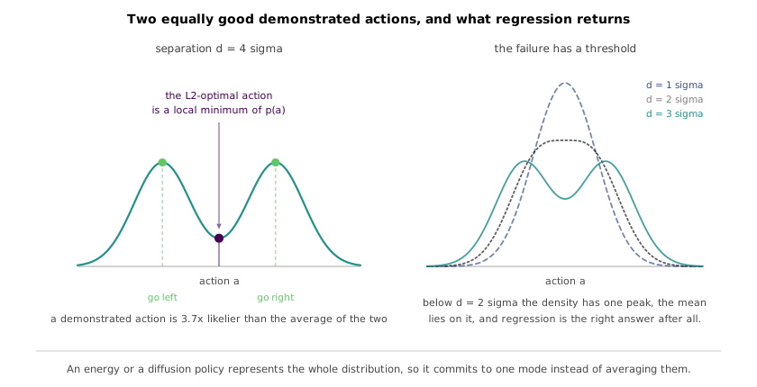
Squared error has a unique minimiser and it is the conditional mean. If the demonstrations at some state are unimodal, that is exactly what is wanted. But human demonstrations are routinely multimodal: shown an obstacle, one demonstrator goes left and another goes right, and both are correct. The conditional mean of go left and go right is go straight, into the obstacle. The regression has not made an error in any sense the loss can see — it has returned the value that minimises expected squared error — and the action it returns is one no demonstrator ever took and no demonstrator would endorse.
It is tempting to leave the claim there, and the claim as stated is not quite true. The generator behind Figure 18.8 makes the toy case explicit: two demonstrated actions at , each Gaussian with standard deviation , mixed with equal weight. The L2-optimal prediction is the mixture mean, which the generator confirms two ways — analytically, and by minimising expected squared error numerically over a grid. But whether that mean is a bad action depends on , and the dependence has a sharp threshold: an equal-weight mixture of two Gaussians is bimodal if and only if . Below that separation the two demonstrations are not distinguishable modes at all, the density has a single peak, and the mean sits on it. Regression is then the right answer.
The threshold is exact and the generator checks it by counting local maxima of the density on a fine grid while sweeping the separation, recovering against the closed-form . Above it, the situation inverts in a way stronger than “the mean is a compromise”: the mean becomes a local minimum of the density. At a demonstrated action is 3.7 times likelier than their average; at it is 45 times likelier. The prediction that minimises squared error is, in its own neighbourhood, the least likely thing to do.
The fix is to stop asking the policy for a single number and ask it for a distribution. Implicit behaviour cloning does this with an energy function: rather than , learn a scalar trained so that demonstrated actions have low energy, and select actions at inference by minimising it,
An energy landscape can have two minima, and the picks one of them rather than averaging them. It also copes with discontinuity: an explicit network is a continuous function of its input and therefore cannot represent a policy that must switch abruptly as the state crosses a boundary, whereas the location of an energy minimum can jump while the energy itself stays smooth.
Diffusion Policy applies the same insight through the machinery of Section 15.6. The policy is a conditional denoising diffusion process over actions: start from noise and iteratively refine it, conditioned on the observation, until it lands on an action. Because a diffusion model represents an arbitrary distribution rather than a point estimate, multimodality is handled by construction, and because Section 15.14’s framing makes it a gradient field being followed rather than a function being evaluated, it scales to the high-dimensional output that the next idea needs. The policy does not predict one action but a short sequence of future actions, executing only the first few before replanning — the receding-horizon idea of Section 18.5 reappearing, but for a different reason: here it buys temporal consistency, since a policy that recommits to a whole plan at every step can dither between two modes, choosing left at one timestep and right at the next and going straight after all. Across 15 tasks from four manipulation benchmarks, this averages a 46.9 % improvement over the previous state of the art, and it works on tasks with genuinely fine-grained contact — spreading butter, peeling a potato, sliding a book onto a shelf.
18.7 Robotic foundation models
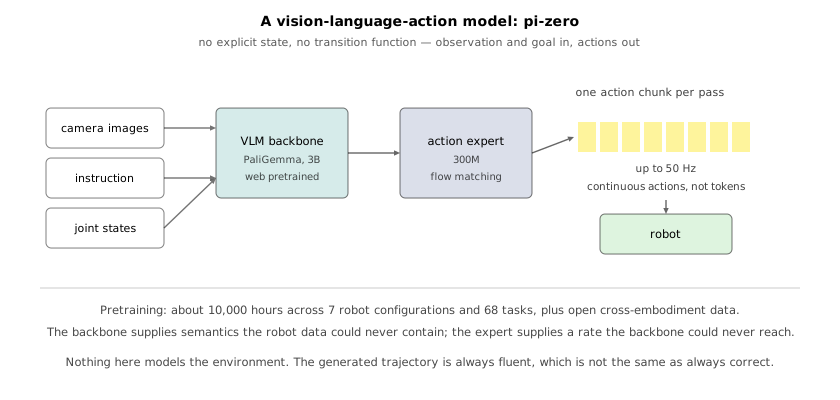
A robotic foundation model is, structurally, the least novel thing in this chapter. It has no explicit state representation and no transition function; it does not model the environment at all. It is a policy mapping an observation and a goal to an action — exactly what Section 18.6 was fitting, trained by exactly the same supervised objective on exactly the same kind of teleoperated demonstrations. What is different is the demand placed on it, and the demand is Section 17.1’s: the same weights should work across many tasks, many objects and many environments, including ones nobody anticipated.
The lecture’s definition of the target is an analogy, and it is a good one because it names both the achievement and the failure mode in the same breath. A vision-language model’s answer may not be correct, but it is always reasonable — fluent, on-topic, plausibly shaped. The corresponding claim for a robot policy is that the synthesised action may not be optimal, but the trajectory will always be smooth, continuous and responsive to the instruction. That is a real property and it is what makes these models feel different from a task-specific policy, which fails by jittering or freezing. It should also be read as a warning, for the same reason the language analogy is apt: a system that always produces something plausible has removed the most reliable signal that it is wrong. The names attached to this class — vision-language-action models, large behaviour models — describe the same object.
The line of work is short and fast. RT-1 in December 2022 established the recipe, and its numbers are the honest measure of what this costs: roughly 130,000 demonstration episodes covering over 700 tasks, collected with a fleet of 13 robots over 17 months. The model itself is small — 35 million parameters, running at 3 Hz — because the constraint is the control deadline of Section 18.2 rather than capacity. RT-2 made the change that matters conceptually: instead of training a policy that happens to consume vision and language, it takes a vision-language model already pretrained on the web and fine-tunes it to emit actions as if they were tokens, co-trained on the original vision-language data so the semantics are not overwritten. What that buys is generalisation that the robot data does not contain — asked to pick up an improvised hammer, it reaches for a rock, because the web taught it what a hammer is for and the robot data only taught it how to pick things up. RT-X and OpenVLA followed, and 2025 brought a crowd of them.
π0 is the one the lecture works through, and its architecture is the clearest statement of what the class has settled on. A pretrained vision-language backbone — PaliGemma, 3 billion parameters — supplies semantics from web-scale data. Bolted to it is a smaller action expert of about 300 million parameters that consumes the backbone’s representation together with the robot’s joint states and emits actions. The action expert does not emit discretised tokens; it produces continuous actions by flow matching, the straight-line variant of diffusion from Section 15.7, and it produces not one action but a chunk of consecutive future actions in a single forward pass, which is what allows control at up to 50 Hz from a 3.3-billion-parameter model. The relationship between the two halves is worth stating plainly, because it is the whole design: the backbone supplies knowledge that no volume of robot data could contain, and the expert supplies a control rate the backbone could never reach. Pretraining used about 10,000 hours of demonstrations across 7 robot configurations and 68 tasks, together with open cross-embodiment data.
The training is split the way language models are, and for the same reason. Pretraining produces a base model broad enough to handle simple tasks that resemble what it has seen. Anything harder — and anything genuinely new — requires post-training on task-specific data. This is not a shortcoming of the particular model; it is the shape of the field. The base model is a prior over reasonable behaviour rather than a solution to any specific task, and the honest reading of the demonstration videos is that the impressive long-horizon results are post-trained. π0.5 extends the claim furthest, cleaning kitchens and bedrooms in homes that were not in its training data, with multi-stage behaviours lasting ten to fifteen minutes.
Two caveats deserve as much attention as the results, and both come from the lecturer rather than from the papers.
The first explains something anyone watching these videos notices, which is that the robots are slow. The reason is not inference latency and not planning. The demonstrations were collected by a human teleoperating the same robot, and teleoperation is slower than using one’s own hands even after hours of practice — the operator is driving an unfamiliar embodiment, at a distance, with occlusions that force them to shift viewpoint before they can tell whether a stage is complete. The policy is therefore imitating a human who has been artificially slowed down, and it inherits that speed exactly. The ceiling is in the data collection process, not in the model, which is why making demonstration collection faster is itself an active research direction rather than an engineering chore.
The second is a limit on the whole approach, and it returns to where this chapter started. Asked whether one large policy will eventually cover a household, the lecturer’s answer is no. Folding a box is already a long-horizon task and it is genuinely impressive that a single policy handles it; but folding shirts and making beds and clearing floors, in an unfamiliar house, is a different kind of problem, and his expectation is that some higher-level abstraction — a scene graph, a symbolic decomposition — will have to sit above the vision-language-action model and steer it. That is the compositional structure of Section 18.5 reappearing at the level of tasks rather than of objects, and it is the same gap the last chapter identified: these models represent entities well and the relations between them poorly, and a policy that must plan across a house is a policy that must reason about relations.
18.8 What is not solved
The most serious unsolved problem in robot learning is not a modelling problem. It is that nobody can measure anything reliably, and this follows from the same closed loop that started the chapter.
Evaluation is conducted in the real world, on real hardware, because nothing else predicts real performance. That makes it expensive and slow: a large laboratory runs a grid of teleoperation rigs for evaluation and waits two days for results, and the description offered of their situation — we have a large enough budget that we can still make progress — is a statement about how the bottleneck is being managed rather than solved. It also makes it noisy in a way that defeats comparison across groups. Two labs evaluating the same policy will get different numbers, because the initial configuration of the objects, the lighting, and the friction of the particular table are all part of the environment, and none of them is written down in a paper.
Underneath that is the deeper problem, and it is the cleanest structural break from every other chapter in this book. The training loss does not predict task success. In supervised learning the validation loss is the thing you care about, up to a generalisation gap; a lower loss is a better model, and the whole methodology of the field rests on that being true. A policy’s training loss measures one-step action prediction accuracy on demonstration data. Task success measures whether a hundred-step rollout, from an initial state the policy chose to enter, accomplishes something. The compounding-error analysis of Section 18.6.1 is exactly why these come apart: a policy with a lower one-step error can have a higher deployed cost if its errors are correlated in the wrong way, and Equation 18.8 says the gap between per-step accuracy and episode cost grows with the horizon. There is no held-out set that fixes this, because the states the policy will be evaluated on do not exist until the policy generates them.
Simulation is the obvious escape and it has not yet worked as one. Large simulated benchmarks exist — BEHAVIOR-1K at Stanford, Habitat 3.0 at Meta — and every one of them inherits the sim-to-real gap of Section 18.4, now in its most demanding form, because a benchmark has to simulate rigid objects, deformable objects and cloth all convincingly enough that the ranking of policies is preserved. Around that sit problems that are unglamorous and genuinely hard: generating enough assets, digitising real environments, procedurally generating scenes that are both realistic and diverse. The property that would make all of it worthwhile is the one thing not yet demonstrated, which is correlation — that a policy which scores better in simulation is actually better on hardware. The comparison the field reaches for is ImageNet, and it is the right one for a precise reason. ImageNet mattered not because the images were interesting but because, for several years, progress on that benchmark was progress in the field. Robot learning has no such object, and building one is arguably a larger contribution than any policy would be.
Three other threads are worth naming as where this goes next.
The first closes a loop within the chapter. The community is collecting action-conditioned interaction data at unprecedented scale in order to train policies — and using it only for policies discards most of what it contains. Every one of those transitions is a statement about how the world responds to being acted on, which is precisely the training signal Section 18.5 needed and never had at scale. A foundation world model, in the sense of action-conditioned future prediction, is the natural other thing to build from the same data, and the open questions about it are the ones this chapter has already met at small scale: should it predict in 3D, how much structural prior should it carry, and how should learning and physics be divided. The interesting prospect is not either artefact alone but the interplay — a policy proposes, a world model evaluates.
The second is that the foundation models being borrowed were not built for this. A language or vision-language model has read a great deal about the world and interacted with none of it, and its understanding of geometry, contact and physical consequence is correspondingly thin. The proposed correction rhymes with how language models were aligned: reinforcement learning from human feedback made models useful by optimising against judgements they could not derive from text, and reinforcement learning from embodied feedback would do the same against outcomes that only the physical world can supply.
The third is that none of this survives as a static artefact. A deployed robot meets new scenarios, users with preferences that differ from the ones in the training data, and its own accumulating experience — so adaptation and lifelong learning are requirements rather than extensions. And every result in this chapter is a systems result before it is a modelling result: delays, compute budgets, and modules that have to talk to each other on a deadline decide what works, and a policy that is correct but late is not a policy.
The chapter began by observing that a robot’s output changes its next input, and every difficulty since has been that fact wearing a different costume. It is why the reward is delayed and the credit ambiguous; why a cloned policy drifts off the distribution it was fitted on; why the training loss stops predicting success; and why evaluation cannot be made cheap by holding data back. Reinforcement learning attacks it with interactions and pays in samples. Model learning attacks it with a predictive model and pays in the difficulty of choosing what to predict. Imitation attacks it with human demonstrations and pays in the cost of collecting them and in the horizon over which small errors grow. Foundation models attack it by borrowing everything the web already knows and paying only for the last mile in robot data. None of them removes the loop, because the loop is what the problem is.