10  Object Detection and Segmentation

Lecture 9

Based on Lecture 9 of CS231n, Stanford University, Spring 2025.

10.1 Past a single label

Every architecture so far has ended the same way. Whatever the network did in the middle — convolve, recur, attend — the last layer produced $C$ numbers, one score per class, and the image was reduced to the index of the largest. That output shape is a strong assumption, and it is wrong for most of what a vision system is asked to do. A photograph of a street does not have a label. It has a road, two pedestrians, a parked car, and a sky, each occupying a particular region, some of them appearing more than once.

Figure 2.9 laid out the four tasks that fall out of relaxing that assumption in different directions, and it is worth restating them in terms of what leaves the network. Classification emits one label for the whole image and keeps no spatial information at all. Semantic segmentation emits a label for every pixel and so retains full spatial detail, but has no notion of objects: two overlapping cats produce one connected region marked cat, and nothing in the output says there were two. Object detection emits a variable-length list of boxes, each with a class, which recovers the count and the rough position but not the shape. Instance segmentation emits a mask per object, which is the union of the last two: it knows there were two cats and it knows which pixels belong to each.

What differs across those four is the shape of the output and the loss that supervises it. What does not differ much is the middle. All four are built on a backbone that turns an image into a stack of feature maps, and by this point in the course that backbone is a settled question — a ResNet, or a Vision Transformer, or whatever the current best classifier happens to be, usually pretrained on a classification task and then adapted. The interesting design work has moved to the ends: how to shape an output that does not have a fixed length, and how to define a loss over it.

That framing also explains why the chapter closes on visualization rather than on another architecture. Once a network is producing spatially structured answers, the question of why it produced them stops being academic. In a medical setting, a model that reports a tumour without indicating where it found the evidence is close to useless, because the radiologist’s job is not to receive the verdict but to check it.

10.2 Labelling every pixel

Take semantic segmentation first, because it is the task whose output shape is least like a classification vector and most like the input. Training data is an image paired with a second image of the same size in which each pixel carries a category index. At test time the network sees a photograph and must produce that second image.

The most direct approach reuses the classifier unchanged. To label a pixel, extract a small patch centred on it, run the patch through a classification network, and take the answer as the label of the centre pixel. The patch is necessary rather than incidental: a single pixel is a colour, and no classifier can say whether a particular brown pixel belongs to a cow or to a fencepost. Only the surrounding region carries the information, so the patch size is a choice about how much context the decision is allowed to consult.

This works and nobody does it, because the cost is prohibitive. One forward pass per pixel means around fifty thousand passes for a modest $224 \times 224$ image, and almost all of that work is redundant — adjacent patches overlap in all but a strip of pixels, so the network recomputes nearly identical features tens of thousands of times.

The redundancy points to its own fix, and the fix is the one convolution was designed for. A convolutional layer already applies the same filter at every spatial position, sharing computation between overlapping receptive fields by construction. If the network contains only convolutional layers — no flattening, no fully connected layers, nothing that destroys the spatial axes — then a $3 \times H \times W$ image passes through to give a $C \times H \times W$ block of scores, one length-$C$ vector per pixel, in a single pass. Taking the argmax over the channel axis at every position yields the $H \times W$ map of predictions.

Training needs no new machinery either. Every pixel is performing a classification, so the loss is the softmax cross-entropy of Section 3.6 evaluated at every position and averaged,

$$L = \frac{1}{HW} \sum_{i=1}^{H} \sum_{j=1}^{W} -\log \frac{\exp\!\big(s_{ij,\,y_{ij}}\big)}{\sum_{c=1}^{C} \exp\!\big(s_{ij,\,c}\big)} \tag{10.1}$$

where $s_{ij,c}$ is the score the network assigns class $c$ at position $(i,j)$ and $y_{ij}$ is that pixel’s ground-truth category. Backpropagation proceeds unchanged. The cost of this arrangement is not in the loss but in the supervision it assumes: Equation 10.1 needs a category for every pixel of every training image, which for years meant somebody tracing object boundaries by hand.

This is the fully convolutional network, and stated that way it looks like the end of the story. It is not, for a reason that is purely about arithmetic. Every layer now operates at the full resolution of the input. A classification network can afford wide layers precisely because it has already thrown away spatial extent by the time the channel count gets large; a $512$-channel feature map at $7 \times 7$ is 25,000 values, while the same 512 channels at $224 \times 224$ is 25 million. Holding full resolution through a deep stack multiplies the cost of every layer by a factor of a thousand or more, and the receptive field grows only as fast as the filters stack, so a network deep enough to see context is also one that cannot be run.

The resolution is the same one the classification architectures reached: downsample. Let the network reduce spatial size as it goes, through pooling or strided convolution, so that the deep layers are cheap and their receptive fields cover most of the image. The difference is that the output must come back out at full resolution, so having gone down, the network has to go back up. That gives the shape almost every dense-prediction model has used since — an encoder that trades resolution for channels and semantic depth, then a decoder that trades them back.

Figure 10.1: The two ways to build a fully convolutional network. Holding the input resolution throughout (top) keeps every prediction aligned with its pixel but makes every layer cost as much as the first. Downsampling and then upsampling (bottom) makes the deep layers cheap and their receptive fields large, at the price of needing an operation that increases spatial size. Drawn for these notes.

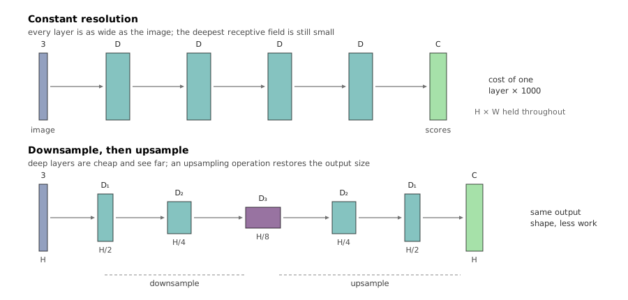
Half of that shape is already familiar. Downsampling is pooling and strided convolution, both covered in Section 6.10. The other half has no counterpart yet: nothing so far in the course takes a small feature map and produces a larger one.

10.3 Putting the resolution back

The simplest upsampling operations have no parameters at all and are worth stating first, because the learnable one is best understood as their generalisation. To double a $2 \times 2$ map to $4 \times 4$, nearest-neighbour unpooling copies each input value into all four output cells that it covers. Bed of nails instead writes each value into one designated cell of its block and leaves the other three at zero, on the argument that subsequent convolutions will spread the value out anyway and the network should choose how rather than have averaging imposed on it.

Both discard something the encoder knew. Max pooling selected a specific position in each window — the location of the largest activation — and then threw that location away. Max unpooling keeps it: each pooling layer records which of its inputs was the maximum, and the corresponding unpooling layer writes its input back to exactly that position, zeroing the rest. Because the indices come from a particular pooling layer, this pairs the encoder and decoder position by position, and the resulting decoder is a mirror image of the encoder rather than an independent stack. What it buys is spatial alignment: an edge that was detected at a specific pixel is restored to that pixel rather than to the corner of a block.

Figure 10.2: Three parameter-free ways to double the spatial size of a feature map. Nearest-neighbour replicates, bed of nails writes one cell per block and zeroes the rest, and max unpooling writes to the position that the paired pooling layer recorded as its maximum — the only one of the three whose output stays aligned with the features that produced it. Drawn for these notes.

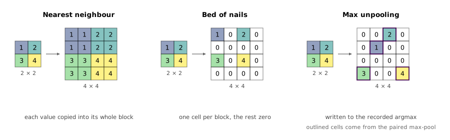
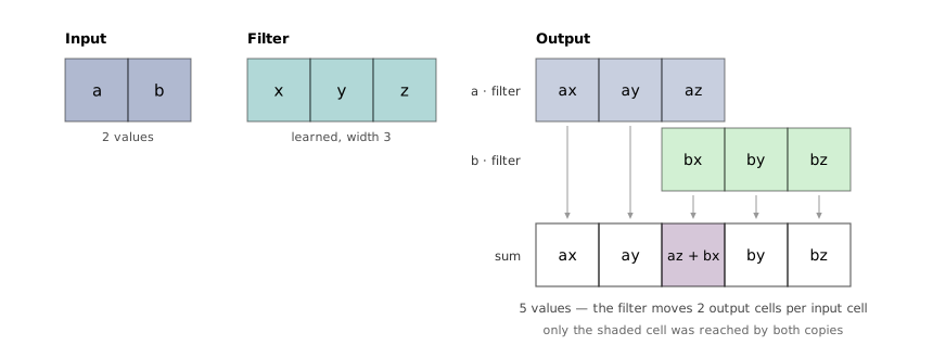
None of the three has a parameter. The learnable version comes from reading strided convolution backwards. In a stride-2 convolution the filter advances two positions in the input for each one position in the output, which is what makes the output half the size; the stride is a ratio between movement in the input and movement in the output. Swap the two. Let the filter advance two positions in the output for each one in the input, and the output comes out twice as large.

The operation that ratio describes is a transposed convolution, and its arithmetic is the reverse of the usual one in a specific sense. An ordinary convolution takes a dot product between the filter and a patch of the input, producing one output number from many input numbers. A transposed convolution takes one input number, multiplies the whole filter by it, and adds the result into a patch of the output — one input number scattering into many. Where the scattered patches overlap, as they must when the filter is wider than the stride, the contributions are summed.

A one-dimensional example makes the whole operation visible. Take an input of two values $a$ and $b$, a filter $(x, y, z)$, and stride 2. The first input contributes $a \cdot (x, y, z)$ starting at output position 0; the second contributes $b \cdot (x, y, z)$ starting at position 2. The output is

$$\big(\,ax,\; ay,\; az + bx,\; by,\; bz\,\big) \tag{10.2}$$

with the sum appearing at the one position both filters reached. The filter weights are learned exactly as any convolution’s are.

Figure 10.3: A stride-2 transposed convolution in one dimension. Each input value scales a copy of the filter, the copies are laid down two output positions apart, and the single position covered by both copies receives their sum, giving Equation 10.2. Drawn for these notes.

The name is the last piece, and it comes from writing convolution as the linear map it always was. A convolution with kernel $(x, y, z)$, stride 1 and one cell of zero padding, applied to a length-4 input, is a matrix product:

$$X\mathbf{a} = \begin{bmatrix} y & z & 0 & 0 \\ x & y & z & 0 \\ 0 & x & y & z \\ 0 & 0 & x & y \end{bmatrix} \begin{bmatrix} a_0 \\ a_1 \\ a_2 \\ a_3 \end{bmatrix} \tag{10.3}$$

Each row of $X$ is the filter shifted to one output position, which is what makes the matrix banded and its entries tied together. Transposed convolution multiplies by $X^{\mathsf{T}}$ instead of $X$ — hence the name, and hence also the older and worse name deconvolution, which the operation does not deserve since it does not invert the convolution, only its shape. The transpose is exactly the matrix that backpropagation through a convolution already uses to send gradients from output to input, so the forward pass of a transposed convolution is the backward pass of an ordinary one.

One consequence of Equation 10.2 is worth knowing before using it. When the filter width is not a multiple of the stride, the output positions receive unequal numbers of contributions — in the example above, position 2 gets two terms and its neighbours one — and a network trained this way tends to produce a regular grid of brighter and darker cells. These checkerboard artifacts are common enough that many current models avoid transposed convolution altogether, upsampling by interpolation and following it with an ordinary stride-1 convolution to do the learning.

10.4 The shape that keeps coming back

Downsampling and upsampling in one network has an unwanted property: the information the decoder needs most is precisely what the encoder was built to discard. The deep layers know what is in the image, because their receptive fields are large and their features abstract. They do not know where very precisely, because eight-fold downsampling has left one feature vector to speak for a $8 \times 8$ block of pixels. Segmentation needs both, and the boundary between a cat and the grass is exactly the place where the coarse answer is worst.

U-Net fixes this by not routing all the information through the bottleneck. At each resolution the encoder’s feature map is copied across and concatenated onto the decoder’s feature map at the same resolution, so the layer that produces the final full-resolution output sees both the upsampled deep features and the original shallow ones, which never lost their spatial precision. The deep path supplies the category and the skip connection supplies the boundary.

Figure 10.4: U-Net. The left branch downsamples and widens, the right branch upsamples and narrows, and at each level the encoder’s feature map is concatenated onto the decoder’s before the next pair of convolutions. Depth carries semantics down the left side; the horizontal copies carry localisation across. Drawn for these notes.

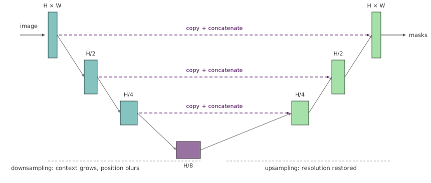
The skip connections are the same device Section 7.8 used, applied for a different reason. In a residual block the shortcut exists so that gradients reach early layers and the identity is easy to represent; here it exists so that high-resolution detail reaches the output without having to survive a round trip through the bottleneck. In both cases the lesson is that a strictly sequential stack forces information through a channel that need not be the only one.

U-Net was published for biomedical segmentation and remains the strongest thing to reach for on a small medical dataset without a foundation model. Its shape also outlived its original purpose entirely: the denoising network at the centre of a diffusion model is a U-Net, for the same structural reason, since predicting noise at every pixel is a dense-prediction problem needing both global context and pixel-accurate output.

What semantic segmentation cannot do, at any level of accuracy, is count. Equation 10.1 labels pixels, and two cats sitting together produce one region marked cat with nothing to indicate that two animals are present. Recovering objects, as opposed to categories, requires an output that is not a map.

10.5 Detection is not a regression problem

Start with the easy case, because it is genuinely easy and it fails in an instructive way. Suppose every image contains exactly one object. Then the output is a class and a box, the box being four numbers $(x, y, w, h)$, and the network needs two heads on a shared backbone: a classification head producing $C$ scores, and a regression head producing four coordinates.

Each head brings its own loss. The class scores take softmax cross-entropy; the coordinates take a regression loss, the squared distance from the ground-truth box. Both are differentiable, so both can be trained at once by adding them,

$$L = L_{\text{cls}}\big(s,\, y\big) + \lambda \, \big\lVert \mathbf{b} - \mathbf{b}^{*} \big\rVert^{2} \tag{10.4}$$

with $s$ the predicted scores, $y$ the true class, $\mathbf{b}$ the predicted box, $\mathbf{b}^{*}$ the true one, and $\lambda$ a hyperparameter setting the exchange rate between the two. This is a multi-task loss, and the pattern — one backbone, several heads, one weighted sum — is how essentially every model in this chapter is trained. The awkward part is $\lambda$: the two terms are measured in different units, so it cannot be reasoned about from first principles and has to be tuned against the metric that is actually cared about.

Now allow more than one object, and the architecture breaks at a level below the loss. An image with one cat needs four numbers plus a class; an image with three needs twelve; a crowd scene needs hundreds. A fully connected output layer has a width fixed when the network is built. There is no value of that width which is right, because the required width is a property of the image, and the network does not know the image when it is compiled.

The obvious workaround is to change what a single prediction is about. Rather than asking the network to describe the image, ask it about a region: given a crop, is this a cat, a dog, or background? That question has a fixed-size answer regardless of how many objects the image contains, and running it over many crops recovers a variable-length result — one detection per crop that came back as a non-background class.

The difficulty moves to which crops. Objects appear at any position, any scale, and any aspect ratio, so an exhaustive sweep is a four-dimensional search whose size grows as roughly the square of the number of pixels. On a $640 \times 480$ image, running a full network on every plausible box is not slow but infeasible, and the sliding-window trick that rescued segmentation does not apply, because the crops here differ in size and must each be resized to the classifier’s fixed input.

10.6 Proposing regions

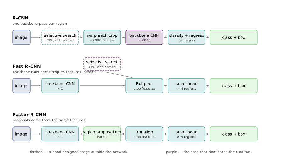
The way out, and the one the field took for most of a decade, is to stop searching exhaustively and get the candidates from somewhere cheaper. Before deep learning was involved at all, there were algorithms for finding image regions that look like they contain some object without knowing which — grouping pixels into blobs by colour and texture, merging them hierarchically, and returning the merged regions as candidates. Selective search is the best known, and it produces roughly two thousand proposals per image in a few seconds on a CPU. That is a reduction of several orders of magnitude from the exhaustive sweep, and it has high recall: the true objects are almost always among the two thousand, buried in a great many false ones the classifier can reject.

R-CNN is the direct application of that idea. Run selective search, warp each proposed region to the fixed $224 \times 224$ input, push it through an ImageNet-pretrained convolutional network, classify the resulting features, and — since the proposal’s box was produced by a colour-and-texture heuristic and will not be tight — also regress four corrections $(\mathrm{d}x, \mathrm{d}y, \mathrm{d}w, \mathrm{d}h)$ that nudge the box onto the object. Using a pretrained classifier as a feature extractor for a task it was not trained for is the transfer-learning argument of Section 7.12, and R-CNN is where it first paid off spectacularly on detection.

It is also unusably slow, for a reason that should look familiar. Two thousand proposals means two thousand independent forward passes per image, and those proposals overlap heavily, so the network recomputes nearly the same features many times over — the same redundancy that made per-pixel classification hopeless in Section 10.2, in a new setting.

And the fix is the same fix. Convolution preserves spatial correspondence: a position in a conv5 feature map corresponds to a known region of the input image. So there is no need to crop the image and then run the network. Run the network once on the whole image, then crop the features. Fast R-CNN does exactly that — one backbone pass per image, a projection of each proposal onto the feature map, a crop, and a small per-region head producing the class and the box offsets. The backbone’s cost is paid once and shared across all two thousand regions; only the small head runs per region. The paper reports training VGG16 nine times faster than R-CNN and testing 213 times faster, at higher accuracy.

Figure 10.5: Three generations of proposal-based detection. R-CNN crops the image and runs a full backbone per region. Fast R-CNN runs the backbone once and crops its features, leaving only a small head per region. Faster R-CNN replaces the external proposal algorithm with a network reading the same features, so nothing outside the model remains. Drawn for these notes.

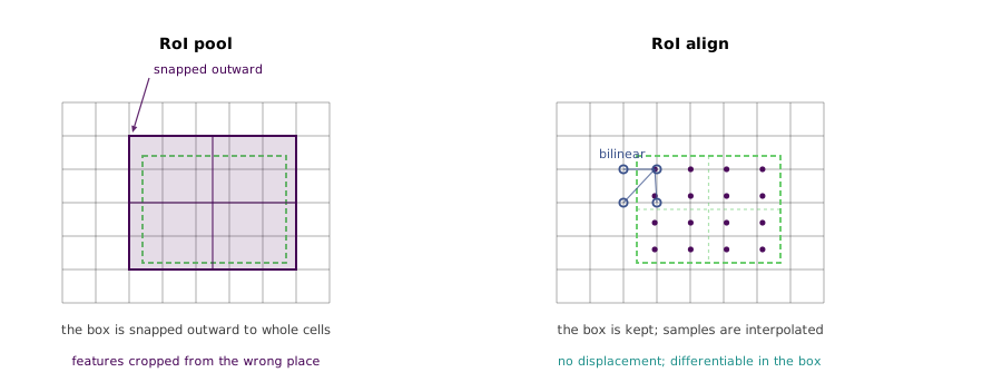
Cropping features is less trivial than cropping pixels, because the proposal’s box is in image coordinates and the feature map is on a coarser grid — a stride-32 backbone means one feature cell per $32 \times 32$ pixel block. RoI pooling handles this by snapping the projected box outward to whole feature cells, dividing the snapped region into a fixed $7 \times 7$ grid of roughly equal subregions, and max-pooling within each. The output is $C \times 7 \times 7$ regardless of the proposal’s size, which is what lets a fixed-width head consume regions of any shape.

The snapping is a real defect, not a rounding detail. A box that should start at feature coordinate 3.4 is treated as starting at 3, displacing the cropped features by up to half a cell — several pixels in the original image — and the subregion boundaries inherit the same error. For a class label this hardly matters. For anything that has to be pixel-accurate, it matters a great deal, which is why it was fixed only when masks arrived. RoI align does not snap. It keeps the box’s real-valued coordinates, samples at regularly spaced points inside each subregion, and computes each sample by bilinear interpolation of the four surrounding feature cells,

$$f_{xy} = \sum_{i,j \in \{1,2\}} f_{ij} \, \big(1 - |x - x_i|\big)\big(1 - |y - y_j|\big) \tag{10.5}$$

where $f_{ij}$ are the features at the four neighbouring grid positions and $(x_i, y_j)$ their coordinates. Every term is differentiable in $x$ and $y$, so gradients flow back through the sampling positions as well as the features.

Figure 10.6: RoI pool against RoI align. Pooling snaps the projected box to feature-cell boundaries, so the cropped region is displaced from the object by up to half a cell; align keeps the real-valued box and reads each sample point by bilinear interpolation from its four neighbours, as in Equation 10.5. Drawn for these notes.

10.7 Learning the proposals

Fast R-CNN made the network cheap enough that the proposal step became the bottleneck. Selective search runs on the CPU and takes about two seconds per image, against a fraction of a second for everything else; the model was now waiting on a hand-designed algorithm from before the deep-learning era, one that cannot be trained and does not improve when the rest of the system does.

Faster R-CNN removes it by predicting proposals from the features the backbone has already computed. The region proposal network is a small convolutional head over the feature map. At each of its spatial positions it considers $K$ anchor boxes — reference rectangles of fixed sizes and aspect ratios, centred on that position — and predicts two things per anchor: an objectness score saying whether the anchor contains an object of any class, and four corrections transforming the anchor towards the true box if it does. For a $512 \times 20 \times 15$ feature map this is a $K \times 20 \times 15$ tensor of scores and a $4K \times 20 \times 15$ tensor of offsets, both produced by ordinary convolutions in one pass on the GPU. Sorting the resulting boxes by objectness and taking the top few hundred gives the proposals, and the paper needs only 300 of them where selective search supplied two thousand.

Anchors deserve a moment, because the device recurs throughout detection. The network is not asked to produce boxes from nothing, which is a hard unconstrained regression; it is asked to classify a fixed set of guesses and to correct the good ones slightly. Regressing a small offset from a nearby reference is a far better-conditioned problem than regressing absolute coordinates, and using $K$ anchors of different shapes at each position means at least one reference is usually close to any given object.

With the RPN in place, Faster R-CNN trains end to end against four losses at once: objectness and box regression in the proposal network, class scores and box regression in the per-region head. It runs at about five frames per second including every step, and the structure has a name — a two-stage detector, in which the first stage runs once per image and the second once per surviving region.

One piece of the pipeline is deliberately not learned. Many anchors near the same object survive, so the raw output contains clusters of near-duplicate boxes for a single thing. Non-maximum suppression removes them: sort detections by score, keep the highest, discard any remaining box overlapping it by more than a threshold in intersection-over-union, repeat. It works, it is universally used, and it is a hand-written procedure with a hyperparameter sitting outside the network — which is exactly the sort of component the rest of this chapter is about absorbing into learning.

10.8 One pass

Two stages means two passes, and the second one runs per region. If the goal is a detector that keeps up with a camera, the natural question is whether the second stage is needed at all — whether the classification could not be done in the same pass that produced the boxes.

YOLO answers that it can, by fixing the set of candidate boxes in advance and predicting everything about them at once. Divide the image into an $S \times S$ grid, $7 \times 7$ in the original. Attach $B$ base boxes to every cell. Then a single fully convolutional pass produces, for each cell, five numbers per base box — four coordinate corrections and a confidence that this box contains an object — and one distribution over the $C$ classes. The output of the whole network is one tensor,

$$S \times S \times \big(5B + C\big) \tag{10.6}$$

and detection is done. There is no proposal stage, no per-region head, and no variable-length intermediate: the network’s output shape is fixed at compile time, and the variable-length answer is recovered afterwards by thresholding on confidence and running non-maximum suppression over what survives.

Figure 10.7: The YOLO output tensor of Equation 10.6. Every grid cell predicts $B$ boxes as offsets from its base boxes, each with a confidence, plus one distribution over classes for the cell. The whole prediction is one forward pass; thresholding and non-maximum suppression turn the fixed-size tensor into a variable-length list of detections. Drawn for these notes.

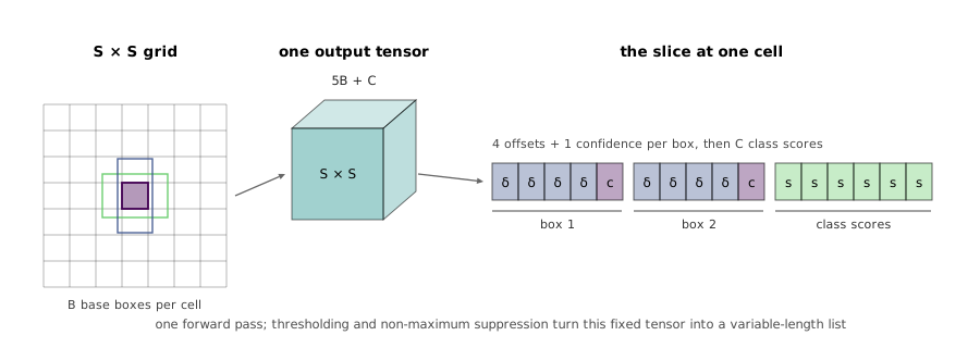
Structurally this is a region proposal network that also predicts categories, with the anchors laid out on a grid instead of being scored and re-cropped. What it buys is speed: the original model ran at 45 frames per second and a reduced version at 155, against Faster R-CNN’s five. What it costs, in that first version, is localisation accuracy — the class distribution is per cell rather than per box, so two objects of different classes in one cell cannot both be reported correctly, and the coarse grid limits how precisely small objects can be placed. Later single-stage detectors (SSD, RetinaNet) closed most of that gap by predicting classes per box and by fixing the class imbalance that dense prediction creates, and the two-stage advantage in accuracy has largely evaporated.

The trade this sets up outlived all the specific architectures. Two-stage detectors spend computation refining a small set of promising regions and are more accurate per unit of accuracy-critical work; single-stage detectors spend a fixed budget everywhere and are faster. YOLO is now many versions past the one described here and remains what most industrial deployments reach for, because in practice latency is a hard constraint and the last point of average precision is not.

10.9 Detection as set prediction

Every detector so far shares two hand-designed components. Anchors encode a prior about what shapes objects take; non-maximum suppression encodes a rule for what counts as a duplicate. Both work, both have hyperparameters, and neither is learned. DETR removes both by changing what the network is asked to produce: not a dense field of scored boxes to be filtered, but a set of exactly $N$ predictions, once, with the network itself responsible for not repeating.

The architecture is the transformer of Section 9.10 with almost nothing added. A convolutional backbone reduces the image to a feature map; the map’s cells become tokens; positional encodings supply the geometry; a transformer encoder mixes them. The decoder is where the new idea sits. Its inputs are $N$ object queries — learned vectors, one per output slot, that are parameters of the model rather than functions of the image. Each query passes through self-attention against the other queries and cross-attention against the encoder output, and the resulting vector goes through a small feed-forward network producing a class and a box. $N$ is fixed and chosen larger than the number of objects any image is expected to contain; the original model used $N = 100$.

Nothing in that description tells a query where to look. The queries begin as arbitrary learned vectors, and what stops all hundred from converging on the same large object in the middle of the image is the self-attention among them: each query sees what the others are proposing and can differentiate itself. Specialisation is a consequence of training rather than a constraint imposed by construction, and after training the individual queries do settle into rough preferences for regions and scales.

The loss is the part that makes this work, and it has to solve a problem the previous detectors never faced. The network emits $N$ predictions in some order; the ground truth is a set of objects in no particular order. There is no natural correspondence between slot 7 and any particular cat, so the loss must first decide which prediction is responsible for which object. DETR does this by finding the cheapest one-to-one assignment — a bipartite matching between the $N$ predictions and the ground-truth objects, padded with a special $\varnothing$ class meaning no object so that both sides have $N$ elements:

$$\hat{\sigma} = \arg\min_{\sigma \in \mathfrak{S}_N} \sum_{i=1}^{N} \mathcal{L}_{\text{match}}\big(y_i,\, \hat{y}_{\sigma(i)}\big) \tag{10.7}$$

where $\sigma$ ranges over permutations of the $N$ slots, $y_i$ is the $i$-th ground-truth element and $\hat{y}_{\sigma(i)}$ the prediction assigned to it, and $\mathcal{L}_{\text{match}}$ scores a pairing by its class probability and box overlap. The minimum is found by the Hungarian algorithm in cubic time, which is negligible for $N = 100$. Having fixed the assignment, the actual training loss is the usual multi-task combination of Equation 10.4 applied to the matched pairs, with unmatched slots supervised towards $\varnothing$.

Figure 10.8: DETR. A backbone and transformer encoder turn the image into a set of tokens; $N$ learned object queries attend to those tokens and to one another, each emitting a class and a box. Training matches the $N$ predictions to the ground-truth objects one-to-one via Equation 10.7, with the unmatched slots supervised towards the no-object class. Drawn for these notes.

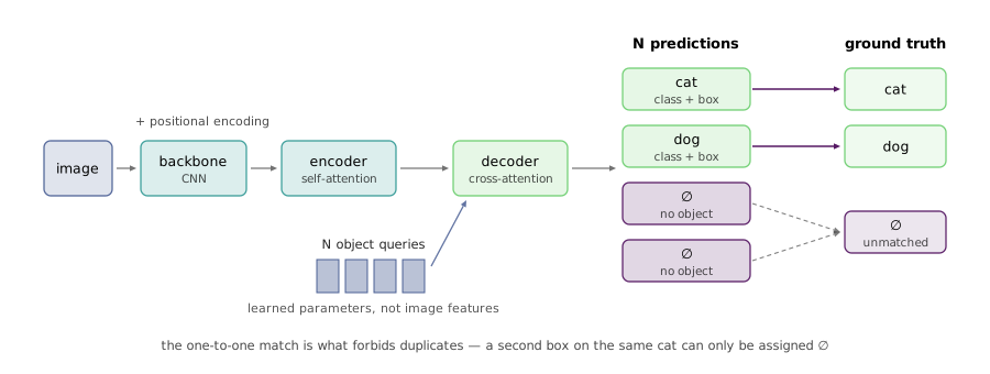
The one-to-one constraint is doing the work that non-maximum suppression used to do. If two slots both predict the same cat, at most one of them can be matched to it and the other is trained to say $\varnothing$ — so producing duplicates is directly penalised, and the model learns not to. Suppression stops being a post-process and becomes a property of the objective.

Two limitations follow from the design and are worth stating. $N$ is a ceiling: an image with more objects than there are queries will have some of them go unreported, and the fix is to train with a larger $N$. And the class list is fixed at training time, as it is for everything else in this chapter — the output is a distribution over known categories plus $\varnothing$, with no mechanism for naming something never seen. Open-vocabulary detection exists, but it works by tying the output to a language embedding rather than to a fixed index, which is a later chapter’s subject.

DETR is five years old and has largely been superseded, its slow convergence in particular having prompted a long line of successors. What it established is durable: detection can be posed as set prediction, and posing it that way removes the last hand-designed stages from the pipeline.

10.10 Instance segmentation for almost free

The fourth task of Section 10.1 is now nearly solved by accident. A detector already isolates individual objects and crops the features belonging to each; a segmentation network already turns features into a per-pixel map. Instance segmentation is what you get by putting the second inside the first.

Mask R-CNN is exactly that. Take Faster R-CNN unchanged, and add a third branch to the per-region head: a few convolutional layers over the RoI features that emit a small binary mask, $28 \times 28$ in the paper, saying which pixels inside the box belong to the object. The multi-task loss of Equation 10.4 gains a third term, a per-pixel binary cross-entropy over the mask.

One detail in that branch is a real design decision rather than a formality. The branch predicts $C$ masks per region — one for every class — and the loss is applied only to the mask for the class the region actually belongs to. The alternative, one mask with a softmax over classes at each pixel, would make the mask branch compete with the classification branch: each pixel would have to decide which class it belongs to as well as whether it is foreground. Decoupling them means the mask branch answers only “is this pixel part of the object”, which is a much easier question, and the paper attributes a substantial part of its accuracy to that choice.

This is also where the misalignment of RoI pooling stops being tolerable. A half-cell shift is invisible in a class label and obvious in a $28 \times 28$ mask stretched back over the object, which is why Equation 10.5 and RoI align were introduced by this paper rather than by Fast R-CNN, whose outputs were coarse enough not to care.

The same branch generalises without modification. Replacing the binary mask with $K$ one-hot maps, one per body joint, and training each with a cross-entropy over its $28 \times 28$ positions turns Mask R-CNN into a pose estimator — the joint is a single pixel that is on, and everything else is off. No part of the architecture changes; only the shape of the target does, which is the chapter’s argument in miniature.

10.11 What has the network learned

Detection and segmentation are what to ask a network for. The rest of the chapter is about what to ask of it: given a trained model and a prediction, what can be said about how it arrived there.

The linear classifier of Section 3.4 was interpretable for free. Each class’s row of $W$ has one weight per pixel, so reshaping the row to the image’s dimensions gives a picture — a template the class score computes an inner product against, showing a blurry front-facing car for the car class and a two-headed smear for horse. That readability came from the model’s weakness: a single linear map from pixels to scores has nowhere to hide.

The first convolutional layer of a deep network keeps that property, for the same reason. Its filters take three input channels, so a $64 \times 3 \times 11 \times 11$ weight tensor is 64 small RGB images and can simply be displayed. Every network trained on natural images produces the same thing there: oriented edges at a range of angles and scales, and blobs of opposing colour. AlexNet, ResNet-18, ResNet-101 and DenseNet learn first layers that are hard to tell apart, which is a strong statement about how little choice there is at that level — and the same family of oriented filters that Section 2.3 found in the visual cortex.

Every layer above the first ends there. A conv2 filter takes 64 input channels, and there is no way to render a $64 \times 5 \times 5$ tensor as something a person can look at. The weights of a deep network are, past the first layer, simply not viewable, and this is the fact that every technique in the remaining sections is working around. What can be examined instead is not the weights but the behaviour: what the network does with a particular image.

10.12 Which pixels mattered

The simplest such question has an answer already sitting in the machinery. Training computes $\partial L / \partial W$, the gradient of a loss with respect to the weights, holding the image fixed. Nothing stops the same backward pass from being run the other way: fix the weights, and compute the gradient of a class score with respect to the pixels,

$$M_{ij} = \max_{c \in \{R,G,B\}} \left| \frac{\partial s_{y}}{\partial I_{ij,c}} \right| \tag{10.8}$$

where $s_y$ is the unnormalized score for the predicted class, $I$ the input image, and the absolute value and maximum over the three colour channels collapse the result to one number per pixel. Simonyan, Vedaldi and Zisserman called the result a saliency map, and its meaning is the ordinary meaning of a derivative: it is large where a small change to that pixel would most change the score. Computing it costs one forward and one backward pass.

The same trick localises intermediate units rather than classes. Pick one channel at one position in a middle layer, treat its activation as the quantity to differentiate, and backpropagate to the image; the result shows what that unit responds to in this particular picture. Plain gradients are noisy for this, so guided backpropagation modifies the backward pass through each ReLU to pass only positive gradients, discarding the negative evidence. The images that come out are dramatically cleaner and the modification is not a derivative of anything — it is a visualization heuristic, and it is worth being clear that this is a different kind of object from Equation 10.8.

That distinction generalises into the main caveat about this whole family of methods. A saliency map looks like an explanation, and the temptation is to accept it as one. Adebayo et al. applied an obvious test — randomise the network’s weights and recompute the map — and found that several popular methods, guided backpropagation among them, produce nearly the same picture from a trained network and an untrained one. A method that cannot distinguish a working model from a random one is showing you image structure rather than model behaviour. Plain gradients pass that test; some of the prettier methods do not.

10.13 Where the evidence is

Saliency works in pixel space and inherits its noise. A different approach works in feature space, using the fact that a convolutional feature map is still laid out over the image: position $(h, w)$ of the last conv layer corresponds to a known region of the input, so a map over those positions can be drawn on the photograph.

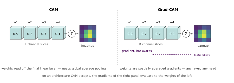
Class activation mapping exploits a particular architecture to make that map fall out of the arithmetic. Suppose the network ends with a $K$-channel feature map $f \in \mathbb{R}^{H \times W \times K}$, a global average pool, and one linear layer with weights $w \in \mathbb{R}^{K \times C}$ — the ending Section 7.8 described, which replaced VGG’s fully connected stack. Then the score for class $c$ is

$$S_c = \sum_k w_{k,c} F_k = \sum_k w_{k,c} \cdot \frac{1}{HW}\sum_{h,w} f_{h,w,k} = \frac{1}{HW}\sum_{h,w} \underbrace{\sum_k w_{k,c}\, f_{h,w,k}}_{M_{c,h,w}} \tag{10.9}$$

where the only step taken is exchanging the two sums. The bracketed quantity $M_{c,h,w}$ is a number per spatial position whose average over positions is the class score, so it decomposes the prediction across the image: it says how much position $(h, w)$ contributed to concluding $c$. Upsampled to the input’s size and drawn as a heatmap, it shows where the evidence for that class was found. Nothing was trained to produce this and no extra computation is needed; it is the score written in a different order.

The catch is the suppose. Equation 10.9 holds only when a global average pool is followed directly by one linear layer, and only for the last convolutional layer. Any other head — a couple of fully connected layers, anything at all between the pool and the scores — and the derivation collapses.

Grad-CAM removes the constraint by noticing what $w_{k,c}$ was doing. It is the sensitivity of the class score to channel $k$, and a sensitivity can always be obtained by differentiation whether or not it happens to be a weight. So pick any layer, with activations $A \in \mathbb{R}^{H \times W \times K}$; compute $\partial S_c / \partial A$ by backpropagation; average it over space to get one number per channel,

$$\alpha_k = \frac{1}{HW}\sum_{h,w} \frac{\partial S_c}{\partial A_{h,w,k}} \tag{10.10}$$

and use those in place of the weights:

$$M^{c}_{h,w} = \operatorname{ReLU}\Big( \sum_k \alpha_k A_{h,w,k} \Big) \tag{10.11}$$

The ReLU is there because only positive contributions are wanted — evidence for class $c$, not against it. On the architecture CAM requires, Equation 10.10 recovers exactly the weights CAM uses, so Grad-CAM is a strict generalisation: any layer, any architecture, including detection and captioning models whose output is not a class score at all.

Figure 10.9: CAM and Grad-CAM. Both weight the channels of a feature map and sum them into a spatial heatmap; they differ only in where the weights come from. CAM reads them off the final linear layer, which requires that layer to exist; Grad-CAM computes them as spatially averaged gradients of the class score, which requires nothing. Drawn for these notes.

Transformers make the whole exercise easier, and that is worth noting as a genuine architectural advantage rather than a footnote. A ViT computes attention weights as part of its forward pass, and those weights are already a distribution over image patches — Section 9.3 showed the same matrices doing the same job for translation. Reading which patches a token attended to needs no gradient, no auxiliary construction, and no architectural assumption; the model reports it. Self-supervised ViTs go further: the attention maps of a DINO-trained model segment the main object of a scene without ever having been shown a segmentation mask, which is a stronger claim about what the model represents than any post-hoc method could establish.

10.14 What this leaves

The chapter’s through-line is that the interesting variable stopped being the architecture. Every model here runs the same backbone — a convolutional network or a ViT, pretrained on classification — and differs in the shape of what leaves it and the loss that supervises that shape. Segmentation makes the output a map and pays for it with upsampling. Detection makes the output a variable-length list and pays for it by predicting against a fixed set of references, whether those are proposals, anchors, grid cells, or queries. Instance segmentation is the two composed, and the composition needed one new operation and no new ideas.

The second thread is what happened to the hand-designed parts, and the sequence is unusually clean. R-CNN learned features but took its regions from selective search. Faster R-CNN learned the regions but kept anchors and non-maximum suppression. DETR removed both, at the cost of needing a loss that solves an assignment problem before it can be evaluated. At each step something that a person had specified was replaced by something the objective specifies instead, and the pattern is worth recognising because it is not finished — the fixed class list is the next such component, and removing it is what vision–language models are for.

The visualization half is a different kind of subject and does not resolve as neatly. The honest summary is that the first layer can be looked at, nothing above it can, and everything else in Section 10.12 and Section 10.13 is an indirect measurement whose validity has to be argued rather than assumed. Grad-CAM is the most useful of them because it makes the fewest architectural demands and because the quantity it computes has a plain reading. The strongest result in the section is not a visualization method at all: it is that attention hands you the map for free, and that a model trained without labels puts it in the right place.

The next chapter adds a dimension. Everything so far has taken a single image; video introduces time, and with it the question of whether motion is a fourth axis to convolve over or something that needs its own machinery.

References

• J. Adebayo et al., “Sanity Checks for Saliency Maps,” NeurIPS, 2018. arXiv:1810.03292
• M. Caron et al., “Emerging Properties in Self-Supervised Vision Transformers,” ICCV, 2021. arXiv:2104.14294
• N. Carion et al., “End-to-End Object Detection with Transformers,” ECCV, 2020. arXiv:2005.12872
• R. Girshick, “Fast R-CNN,” ICCV, 2015. arXiv:1504.08083
• R. Girshick, J. Donahue, T. Darrell and J. Malik, “Rich Feature Hierarchies for Accurate Object Detection and Semantic Segmentation,” CVPR, 2014. arXiv:1311.2524
• K. He, G. Gkioxari, P. Dollár and R. Girshick, “Mask R-CNN,” ICCV, 2017. arXiv:1703.06870
• T.-Y. Lin et al., “Focal Loss for Dense Object Detection,” ICCV, 2017. arXiv:1708.02002
• W. Liu et al., “SSD: Single Shot MultiBox Detector,” ECCV, 2016. arXiv:1512.02325
• J. Long, E. Shelhamer and T. Darrell, “Fully Convolutional Networks for Semantic Segmentation,” CVPR, 2015. arXiv:1411.4038
• A. Odena, V. Dumoulin and C. Olah, “Deconvolution and Checkerboard Artifacts,” Distill, 2016. doi:10.23915/distill.00003
• J. Redmon, S. Divvala, R. Girshick and A. Farhadi, “You Only Look Once: Unified, Real-Time Object Detection,” CVPR, 2016. arXiv:1506.02640
• S. Ren, K. He, R. Girshick and J. Sun, “Faster R-CNN: Towards Real-Time Object Detection with Region Proposal Networks,” NeurIPS, 2015. arXiv:1506.01497
• O. Ronneberger, P. Fischer and T. Brox, “U-Net: Convolutional Networks for Biomedical Image Segmentation,” MICCAI, 2015. arXiv:1505.04597
• R. R. Selvaraju et al., “Grad-CAM: Visual Explanations from Deep Networks via Gradient-Based Localization,” ICCV, 2017. arXiv:1610.02391
• K. Simonyan, A. Vedaldi and A. Zisserman, “Deep Inside Convolutional Networks: Visualising Image Classification Models and Saliency Maps,” ICLR Workshop, 2014. arXiv:1312.6034
• J. T. Springenberg, A. Dosovitskiy, T. Brox and M. Riedmiller, “Striving for Simplicity: The All Convolutional Net,” ICLR Workshop, 2015. arXiv:1412.6806
• J. R. R. Uijlings, K. E. A. van de Sande, T. Gevers and A. W. M. Smeulders, “Selective Search for Object Recognition,” IJCV 104(2):154–171, 2013. doi:10.1007/s11263-013-0620-5
• M. D. Zeiler and R. Fergus, “Visualizing and Understanding Convolutional Networks,” ECCV, 2014. arXiv:1311.2901
• B. Zhou, A. Khosla, A. Lapedriza, A. Oliva and A. Torralba, “Learning Deep Features for Discriminative Localization,” CVPR, 2016. arXiv:1512.04150