3  Image Classification with Linear Classifiers

Lecture 2

Based on the lecture by Fei-Fei Li and Ehsan Adeli — CS231n, Stanford University, Spring 2025.

3.1 The semantic gap

Image classification asks for a function that maps an image to one label from a fixed set: cat, dog, truck, plane, and so on. The request sounds like ordinary sorting—inspect an object, identify its category—but the input available to a computer is not an object. It is a tensor of numbers. An RGB image of width $W$ and height $H$ is an array in $\mathbb{R}^{H \times W \times 3}$, with each entry usually representing an intensity between 0 and 255. The category is not written anywhere in that array. It has to be inferred.

The difference between the representation and the meaning is the semantic gap. A small change in the scene can change nearly every pixel while leaving the label intact: moving the camera changes the viewpoint, a cloud changes the illumination, and a different background changes many more pixels than the object itself. Objects can be partly hidden, deformed, or surrounded by clutter. A category also contains large intra-class variation: two dogs can differ in pose, breed, scale, and colour more than a dog resembles another dog in a particular image. Context can help or mislead as well. A small object may be hard to recognise in isolation but obvious in a familiar scene.

There is no short collection of rules that solves all of these cases. One can write an edge detector—Canny’s formulation is a canonical example—and detect corners or contours, but the step from local structure to “this is a cat” requires choices about which structures matter and how they combine. The data-driven approach changes the question. Instead of programming a recognition procedure directly, collect labelled examples, fit a classifier to them, and measure its predictions on images it has not seen.

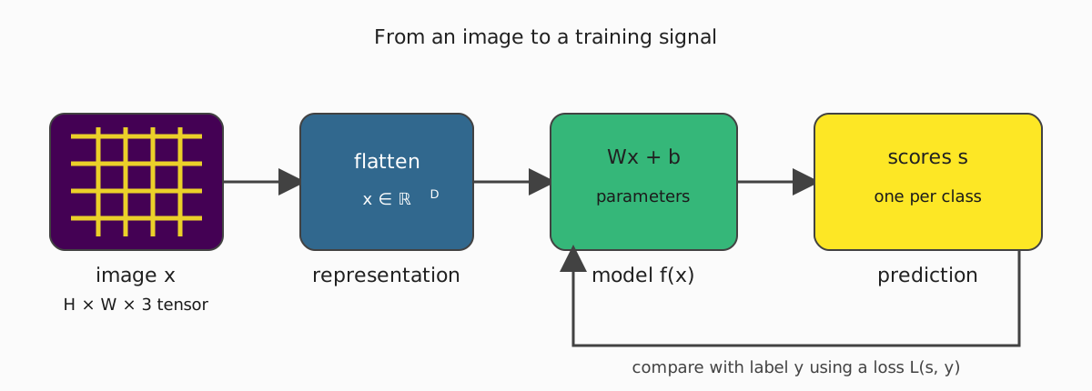
That separation introduces three objects that will recur throughout the course. A model maps an input to a prediction. A loss function says how unsatisfactory that prediction is for a labelled example. An optimization procedure changes the model’s parameters to reduce the average loss on the training set. Figure 3.1 shows how these pieces connect, and the first two classifiers in this lecture make the contrast between the choices explicit.

Figure 3.1: Training separates the representation of an image, the model that produces class scores, and the loss that compares those scores with the label. The same separation will let us replace the linear model with a neural network without changing the basic training logic. Drawn for these notes.

3.2 Nearest neighbors: let the dataset do the work

The nearest-neighbor classifier stores every training image and its label. Given a new image $x$, it compares $x$ with each stored image, finds the closest one under a chosen distance, and returns that image’s label. With a training set $\{(x_i,y_i)\}_{i=1}^N$, the rule is

$$\hat y(x) = y_{\arg\min_i d(x,x_i)}. \tag{3.1}$$

For images, the simplest distance is the $L_1$ or Manhattan distance. If images are flattened into vectors, it is

$$d_1(x,z) = \sum_{p=1}^{D} |x_p-z_p|, \tag{3.2}$$

where $D = H \times W \times 3$ is the number of scalar pixels. The $L_2$ distance instead measures the Euclidean distance,

$$d_2(x,z) = \sqrt{\sum_{p=1}^{D}(x_p-z_p)^2}. \tag{3.3}$$

Nearest neighbors are useful because they reveal what a data-driven method means in its most literal form: the classifier does not learn a compact description of a class; it relies on the training set as a memory. That makes training almost free—there is nothing to fit—but makes prediction expensive. To classify one test image, the algorithm must compare it against all $N$ training images, so prediction costs $O(ND)$ in a direct implementation. In machine learning it is usually acceptable for training to be slow if the resulting model predicts quickly; nearest neighbor has the opposite trade-off.

The $k$-nearest-neighbor variant reduces sensitivity to the one accidental match that Equation 3.1 rests on. It finds the $k$ closest examples and predicts the majority label among them. The integer $k$ and the distance metric are hyperparameters: choices about how the algorithm should operate, rather than parameters inferred from the labelled examples. A larger $k$ smooths over individual examples but can erase small classes or local structure.

This baseline also exposes why raw pixel distances are a poor notion of visual similarity. A one-pixel translation, a tint, or an occluder can produce a large numerical change even when a person would regard the image as the same object. Conversely, two images with similar low-level statistics may depict different categories. The problem is not that Equation 3.2 is badly implemented, and switching to Equation 3.3 does not repair it. The representation and metric have failed to express the invariances that recognition needs.

3.3 Validation is part of the method

Hyperparameters cannot be selected by minimizing training error. With $k=1$, every training image is its own nearest neighbor, so the training accuracy is perfect even if the classifier generalizes badly. Choosing the setting that performs best on the test set is also invalid: the test set would then influence the method, and its final accuracy would no longer be an honest estimate of performance on new data.

The usual division is into training, validation, and test sets. Training examples define the fitted model; the validation set chooses among hyperparameters such as $k$ and the distance; the test set is held back until the end. The validation score estimates how each choice generalizes while preserving the test set as an untouched measurement.

When data are scarce, cross-validation gives a less noisy estimate. Split the training data into $F$ folds, then repeat the following $F$ times: hold out one fold, fit on the remaining $F-1$, and score the held-out fold. Averaging the $F$ scores measures a hyperparameter setting on every training example in turn rather than on one arbitrary split. This costs $F$ times the computation and is uncommon for large deep-learning training runs, but it is a sensible way to compare a few choices on a small dataset such as CIFAR-10. CIFAR-10 contains 60,000 colour images in ten classes, conventionally divided into 50,000 training and 10,000 test examples (Krizhevsky, 2009).

The workflow matters beyond nearest neighbors. A model can always be made to look better on data that helped choose it. Validation protects against that circularity, while the test set answers the narrower question we actually care about: after all choices have been made, how well does the finished procedure work on unseen examples?

3.4 A parametric model: one matrix, one score per class

Nearest neighbors retain all examples. A parametric classifier takes the opposite approach: it compresses the training set into a fixed collection of parameters. Flatten an image into $x \in \mathbb{R}^{D}$, let there be $C$ classes, and define

$$f(x,W,b) = W x + b, \tag{3.4}$$

where $W \in \mathbb{R}^{C \times D}$ is the weight matrix and $b \in \mathbb{R}^{C}$ is the bias vector. The output $s=f(x,W,b)$ contains one score $s_j$ for each class $j$; prediction chooses the largest score, $\hat y=\arg\max_j s_j$.

For CIFAR-10, $D=32\cdot32\cdot3=3072$ and $C=10$, so the matrix in Equation 3.4 has shape $10\times3072$. Each row of $W$ can be viewed as a template for one class: the class score is a weighted sum of image pixels, plus its bias. In this view, positive weights favour pixels or colour channels at particular positions, while negative weights suppress them. The geometric view says the same thing differently. Each class wins in a region of pixel space separated from other regions by hyperplanes, because equality of two class scores gives a linear boundary.

This explains both the appeal and the limitation of the model. It is compact and fast: one matrix multiplication produces all class scores. But one linear boundary cannot express arbitrary arrangements of examples. A class occupying two disconnected regions, a ring surrounding another class, or several distinct visual modes cannot generally be separated from its competitors by a single set of linear score comparisons. Flattening the image also discards the spatial structure that makes nearby pixels and repeated patterns meaningful. Later architectures will address those limitations by composing many learned transformations; for now, the point is to understand how a simple model is trained.

3.5 The loss turns “good” into a number

The classifier is not defined by the score function alone. Many different matrices $W$ and biases $b$ produce different scores, and we need a criterion for preferring one parameter setting to another. Given labelled examples $(x_i,y_i)$, define a per-example loss $L_i$ and average it over the dataset:

$$L(W,b) = \frac{1}{N}\sum_{i=1}^{N} L_i\bigl(f(x_i,W,b),y_i\bigr). \tag{3.5}$$

The loss is deliberately separate from the model. The linear map says what scores can be represented; the loss says which score vectors are desirable. Everything that follows in this lecture fills in the single term $L_i$ inside Equation 3.5, and training becomes the optimization problem of finding parameters with small $L(W,b)$. Regularization and optimization, which the next lectures develop, add further structure to this objective; the present lecture concentrates on the data term.

3.6 Softmax: scores as a probability distribution

The softmax classifier interprets the linear scores as unnormalized log-probabilities, or logits. For score vector $s$, it defines

$$p_j = \frac{\exp(s_j)}{\sum_{k=1}^{C}\exp(s_k)}. \tag{3.6}$$

Every $p_j$ produced by Equation 3.6 is nonnegative and the probabilities sum to one. The predicted class is still the class with the largest score, because exponentiation and normalization preserve the ordering. The extra interpretation is useful for training: if the correct class is $y_i$, the cross-entropy loss is the negative log probability assigned to it,

$$L_i = -\log p_{y_i} = -\log\left(\frac{\exp(s_{y_i})}{\sum_{j=1}^{C}\exp(s_j)}\right). \tag{3.7}$$

Equation 3.7 is small when the correct class receives nearly all the probability and grows without bound as its probability approaches zero. Minimizing the average cross-entropy is equivalent to maximizing the likelihood of the observed labels under the model. It is also the cross-entropy between the one-hot target distribution and the predicted distribution.

At initialization, if all scores are approximately equal, each class receives probability $1/C$. The initial loss is therefore

$$L_i=-\log(1/C)=\log C. \tag{3.8}$$

For ten classes this is approximately $2.3$. This is a useful sanity check: a randomly initialized ten-way classifier should begin near the loss of a uniform guess, not near zero. In numerical code, the softmax is evaluated with a stabilized form—subtracting the largest score before exponentiating—because the probabilities do not change when the same constant is subtracted from every score, while the exponentials become safer to compute.

3.7 Multiclass SVM loss: enforce a margin

The multiclass SVM loss does not ask for calibrated probabilities. It asks for a margin: the correct class should score at least $\Delta$ more than every incorrect class. For an example with score vector $s$ and label $y_i$, define

$$L_i = \sum_{j\ne y_i}\max\left(0,\,s_j-s_{y_i}+\Delta\right). \tag{3.9}$$

The term for class $j$ is zero when the correct score beats it by at least $\Delta$. Otherwise, the term is the amount by which the margin is violated. The loss is therefore piecewise linear: once all constraints are satisfied, increasing the correct score further does not improve the data loss. Piecewise linear also means not differentiable everywhere—each hinge has a corner at the point where its margin is met exactly—so optimization uses a subgradient there. In practice one picks either side of the corner, and the choice rarely matters, because exact ties are unusual in floating-point scores.

A worked example makes the arithmetic concrete. Take three training images, three classes, and $\Delta=1$, with the scores some particular $W$ assigns. For the cat image the scores are $3.2$ for cat, $5.1$ for car, and $-1.7$ for frog. The correct class is cat, so the car term is $\max(0,5.1-3.2+1)=2.9$ and the frog term is $\max(0,-1.7-3.2+1)=0$, giving $L_i=2.9$—the car class outscores the correct one, and the loss is exactly the amount by which that margin is violated. For the car image the scores are $1.3$, $4.9$, and $2.0$; the correct class leads both competitors by more than $\Delta$, both terms vanish, and $L_i=0$. For the frog image the scores are $2.2$, $2.5$, and $-3.1$, and the correct class comes last by a wide margin: the terms are $\max(0,2.2+3.1+1)=6.3$ and $\max(0,2.5+3.1+1)=6.6$, so $L_i=12.9$. Averaging the three gives the dataset objective, $L=(2.9+0+12.9)/3\approx5.27$.

The same sanity check that Equation 3.8 provides for softmax is available here. If the weights are initialized small enough that every score is approximately zero, each of the $C-1$ incorrect classes contributes $\max(0,0-0+\Delta)=\Delta$, so the loss at the first iteration should be close to

$$L_i \approx (C-1)\,\Delta. \tag{3.10}$$

For ten classes and $\Delta=1$ that is about $9$. A first measurement far from this value points to a bug in the implementation rather than to an unlucky initialization.

The loss has a useful invariance. Adding the same constant to every score leaves each difference $s_j-s_{y_i}$ unchanged, so it leaves Equation 3.9 unchanged. Softmax probabilities have the same invariance: their common factor cancels during normalization. What matters in both cases is the relative arrangement of the class scores, not their absolute origin.

The two objectives differ in what happens after a prediction is already correct. SVM stops caring once the margin is met. Softmax continues to reward a larger probability for the correct class, pushing the distribution toward greater confidence. That does not make one universally correct and the other universally wrong; it means they encode different preferences about the scores.

3.8 Softmax and SVM are choices above the same model

Softmax and SVM can be applied to the same linear score function $Wx+b$. They differ in the loss layer, not in the basic model that converts pixels to scores. In practice they may produce similar predicted labels, especially when the data are easy, even though the numerical objectives behave differently. A score vector that already separates the correct class by a large margin can have zero SVM loss while still changing the softmax loss if its confidence changes.

This separation is the main conceptual handoff to the next lectures. A classifier is not just an architecture name. It is a chain of decisions: how the image is represented, how parameters map it to scores, how scores are judged against labels, and how parameters are optimized. Nearest neighbor made the training set itself the model. The linear classifier compresses the examples into $W$ and $b$. Softmax and SVM then impose different notions of what those scores should mean. Once these layers are kept distinct, improving a vision system becomes a tractable question: which part of the chain is limiting the result, and what evidence would tell us that?

References

• J. Canny, “A Computational Approach to Edge Detection,” IEEE Transactions on Pattern Analysis and Machine Intelligence, 8(6), 1986. doi:10.1109/TPAMI.1986.4767851
• A. Krizhevsky, “Learning Multiple Layers of Features from Tiny Images,” Technical Report, University of Toronto, 2009. Report