15  Generative Models II

Lecture 14

Based on Lecture 14 of CS231n, Stanford University, Spring 2025.

15.1 A model defined only by its sampler

The previous chapter closed on a dilemma. An autoregressive model gives an exact likelihood and sharp samples but needs one network pass per subpixel, so producing a megapixel image is three million sequential forward passes. A variational autoencoder samples in a single pass and hands you a latent code, but it is trained through a Gaussian reconstruction term that rewards hedging, and hedging over images means averaging them, which is what blur is. Both failures trace back to the same commitment: both models are trying to put a number on $p(x)$, and the number is what costs them.

Generative adversarial networks abandon the number. There is no expression for $p_\theta(x)$ anywhere in a GAN, no bound on it, and no way to ask the trained model how probable a particular image is. What the model provides is a procedure for producing samples, and nothing else. This is the position at the far right of the taxonomy in the previous chapter: an implicit density model, one that defines a distribution the way a physical process does, by generating from it rather than by describing it.

The mechanics are the same as a variational autoencoder’s decoder, stripped of everything else. Fix a prior $p(z)$ that you chose yourself and can sample from — a unit Gaussian, in practice always. Sample $z \sim p(z)$, push it through a network, and call the output an image:

$$x = G(z), \qquad z \sim p(z). \tag{15.1}$$

The network $G$ is deterministic; all the randomness enters through $z$. Because $G$ is a fixed function, pushing the prior through it induces a distribution over images, written $p_G$, whose density nobody can write down — it would require inverting $G$ and tracking how the map compresses and stretches volume, and $G$ is neither invertible nor volume-preserving. That inability is not an inconvenience to be worked around later. It is the whole design. The generator is free to concentrate its output onto a thin, curved, disconnected region of image space, and it pays no penalty for doing so, because no term in its objective ever evaluates a density.

The goal is stated distributionally: make $p_G$ match $p_{\text{data}}$. If they match, then sampling $z$ and running one forward pass gives a genuine sample from the data distribution, at the cost of exactly one network evaluation. What is missing is any way to measure whether they match, since the whole point was that neither density is available. A maximum-likelihood objective is out of reach by construction. Something else has to supply the training signal.

15.2 The discriminator is the loss function

The answer is to stop writing the objective down and train a second network to be it. A discriminator $D$ takes an image and returns the probability that the image came from the dataset rather than from the generator, so $D(x) = 1$ means real and $D(x) = 0$ means fake. It is an ordinary binary classifier, trained on an ordinary cross-entropy loss, over a dataset half of which is the real training set and half of which is whatever the generator is currently producing.

The two networks are trained against each other on a single scalar quantity:

$$\min_G \max_D \; V(G, D) = \mathbb{E}_{x \sim p_{\text{data}}}\big[\log D(x)\big] + \mathbb{E}_{z \sim p(z)}\big[\log\big(1 - D(G(z))\big)\big]. \tag{15.2}$$

Read Equation 15.2 twice, once from each side, because it means different things depending on which network you hold fixed. Hold $G$ fixed and it is the discriminator’s problem. The first term is large when $D(x)$ is near one on real images; the second is large when $D(G(z))$ is near zero on generated ones. Maximising their sum is exactly binary cross-entropy with the labels real and fake, written without the usual minus sign. Now hold $D$ fixed and read it as the generator’s problem. The first term contains no $G$ and is a constant to it. The second term is small when $D(G(z))$ is near one, so minimising drives the generator towards images the current discriminator calls real.

Figure 15.1: The game and the two gradient paths. The discriminator sees both streams and is trained on the ordinary two-class objective; the generator sees only the fake stream and only through the discriminator. The dashed path is the whole of the generator’s training signal: there is no reconstruction term, no likelihood, nothing anchoring the generator to any particular training image. Backpropagation runs from the discriminator’s output through the generated image and into the generator’s weights, which is why $D$ must be differentiable and why the game is trained end to end.

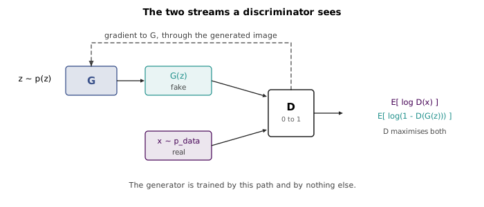
Training alternates. Take an ascent step on $D$ to sharpen the current loss, then a descent step on $G$ against that sharpened loss, and repeat. The intuition is an arms race: as the discriminator gets better at spotting the artefacts of generated images, the only way for the generator to keep scoring is to stop producing them.

The most important structural fact about Equation 15.2 is easy to skip past. $V$ is not a loss. Its value at any moment is a joint property of two networks and says nothing about the quantity anyone cares about, which is how close $p_G$ has come to $p_{\text{data}}$. A weak generator against a weak discriminator and a strong generator against a strong discriminator produce the same numbers. Every other model in this course comes with a curve that goes down when things are going well; a GAN does not, and the practical consequence is that the standard method of debugging a training run — look at the loss — is unavailable. You look at samples, by eye, and that is most of what you have.

15.3 The gradient the obvious objective does not deliver

Consider the beginning of training, when both networks are random. The generator emits noise, and telling noise apart from photographs is trivial, so within a few hundred iterations the discriminator is confident and $D(G(z))$ sits close to zero on everything the generator makes. This is precisely the regime in which the generator most needs a gradient, and it is precisely the regime in which Equation 15.2 stops providing one.

To see why, the derivative has to be taken with respect to the right variable. The discriminator’s final layer is a sigmoid, $D = \sigma(s)$, and the generator influences $D$ only through the pre-sigmoid score $s$, so the quantity that determines how much signal reaches the generator’s weights is the derivative of its loss with respect to $s$. For the objective as written, the generator minimises $\log(1 - \sigma(s))$, and

$$\frac{\partial}{\partial s} \log\big(1 - \sigma(s)\big) = -\sigma(s) = -D. \tag{15.3}$$

The gradient is proportional to $D$ itself. When the discriminator is confident and $D \approx 0$, the gradient is approximately zero: the generator receives almost nothing exactly when it is worst and has the most to learn. The loss curve is flat in the region where training starts, and the game stalls before it begins.

The fix is a change of objective for the generator alone. Instead of minimising $\log(1 - D(G(z)))$, minimise $-\log D(G(z))$. Both are minimised by driving $D(G(z))$ to one, so they express the same wish, but they express it with different curvature:

$$\frac{\partial}{\partial s} \big[-\log \sigma(s)\big] = -\big(1 - \sigma(s)\big) = -(1 - D). \tag{15.4}$$

Now the gradient is proportional to $1 - D$, and it is largest when the discriminator is most confident. The two expressions are mirror images, and at $D = 0.01$ the ratio between them is $99$: the modified objective delivers ninety-nine times the gradient in the regime where training actually begins. This is the non-saturating generator loss, and it is not an optional refinement. A GAN trained from scratch on Equation 15.2 as literally written usually does not train at all.

Figure 15.2: The two generator objectives and what they deliver. The left panel plots each loss against the discriminator’s current output on generated images; both fall as $D(G(z))$ rises, so both encode the same preference. The right panel plots the magnitude of each loss’s gradient with respect to the discriminator’s pre-sigmoid score, which is the signal that actually reaches the generator. Training starts at the left edge, where the confident discriminator puts $D(G(z))$ near zero, and there the two curves differ by two orders of magnitude. The saturating loss is flat where the generator is worst; the non-saturating one is steepest there.

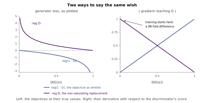
Note what has been given up to get this. The two networks are no longer optimising a single shared quantity — the discriminator maximises Equation 15.2 while the generator minimises something else — so the tidy minimax formulation is already a description of a game nobody plays. Whatever guarantees attach to Equation 15.2 attach to a training procedure that is not the one in use.

15.4 What the game would converge to

There is a reason to believe Equation 15.2 is the right game and not an arbitrary one, and it comes from solving the inner maximisation exactly. For a fixed generator, the discriminator’s problem decouples across images: at each $x$ it is choosing a single number to maximise $p_{\text{data}}(x) \log D(x) + p_G(x) \log(1 - D(x))$, and differentiating that scalar expression gives the optimum immediately,

$$D_G^*(x) = \frac{p_{\text{data}}(x)}{p_{\text{data}}(x) + p_G(x)}. \tag{15.5}$$

The optimal discriminator does not learn features of real images. It reports a ratio of densities — one half wherever the two distributions agree, near one where only real data lives, near zero where only generated data lives. It is also, as the lecture notes, a formula you can write and never evaluate: computing it needs $p_{\text{data}}$, and if you had $p_{\text{data}}$ you would not be training a generative model.

Substituting Equation 15.5 back into Equation 15.2 turns the game’s value into a divergence. Adding and subtracting $\log 2$ inside each expectation converts the two terms into Kullback–Leibler divergences against the mixture $m = \tfrac{1}{2}(p_{\text{data}} + p_G)$, and what is left is

$$V(G, D_G^*) = 2\, D_{\mathrm{JS}}\big(p_{\text{data}} \,\|\, p_G\big) - \log 4, \tag{15.6}$$

where $D_{\mathrm{JS}}(p \| q) = \tfrac{1}{2} D_{\mathrm{KL}}(p \| m) + \tfrac{1}{2} D_{\mathrm{KL}}(q \| m)$ is the Jensen–Shannon divergence. It is non-negative and zero only when its arguments are equal, so the outer minimisation is solved uniquely at $p_G = p_{\text{data}}$, and the value there is $-\log 4 \approx -1.386$.

Figure 15.3: The optimal discriminator and the identity it satisfies, on a one-dimensional problem where every quantity is closed form. The left panel shows a bimodal data density and a Gaussian generator distribution; the right shows $D^*$ from Equation 15.5, which crosses one half exactly where the densities cross and saturates wherever one distribution has the field to itself. The generator’s script evaluates both sides of Equation 15.6 by numerical integration and asserts they agree, then sweeps the generator’s mean to confirm the value bottoms out at $-\log 4$ when the two distributions are made identical.

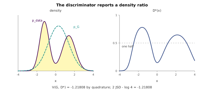
This result is worth understanding for what it does not say. It assumes both networks have unlimited capacity, so that the discriminator can actually reach Equation 15.5 and the generator can represent $p_{\text{data}}$ exactly; real networks are finite and can do neither. It assumes the inner maximisation is solved before every generator step, whereas practice takes one discriminator step per generator step and the discriminator trails behind a moving target. It says nothing about convergence — alternating gradient steps on a saddle point are not guaranteed to find it, and frequently orbit it instead. And, as the previous section established, the generator is minimising a different objective than the one the theorem is about. What survives is real but modest: the game has a sensible unique optimum, which is more than can be said for an arbitrary adversarial loss.

15.5 What GANs turned out to give, and what they cost

Both networks are convolutional in every implementation that mattered; GANs fell out of use before vision transformers arrived. The first architecture to produce non-trivial samples was DC-GAN, a five-layer fully convolutional generator with no pooling and no fully connected layers, and the family peaked with StyleGAN, which injects the latent code not at the input but at every layer through adaptive instance normalisation. Each layer normalises its activations and then rescales them with a per-channel scale $w_i$ and shift $b_i$ predicted from the latent:

$$\mathrm{AdaIN}(x, w, b)_i = w_i \frac{x_i - \mu(x)}{\sigma(x)} + b_i. \tag{15.7}$$

Feeding the latent in at every resolution rather than only at the bottom is what gives StyleGAN its control over coarse and fine attributes separately, and its samples were, for several years, the best images any generative model produced.

The property that made GANs interesting beyond sample quality is that their latent space turned out to be smooth. Draw two codes $z_0$ and $z_1$, interpolate between them, and decode along the path: the images morph continuously, passing through intermediate states that are themselves plausible images rather than superpositions of the endpoints. Nothing in Equation 15.2 asks for this. The lecture makes the point sharply with a counterexample — a generator that ignored $z$ entirely and memorised ten training images would fool a discriminator perfectly well, placing all its mass on ten spikes and leaving the latent space meaningless. Smoothness is an empirical consequence of training a continuous network under pressure to cover the data, not a guarantee.

The costs are three, and they compound. The first is that there is no encoder. The generator maps $z \to x$ and nothing maps back; a GAN cannot tell you the code for a given image except by numerical inversion after the fact. The discriminator enforces only that the distribution of outputs matches the distribution of data, with no correspondence between any particular $z$ and any particular training image, which is a strictly weaker relationship than a variational autoencoder’s.

The second is mode collapse, the failure the memorisation counterexample gestures at. Because no term in the objective is a density, nothing penalises the generator for ignoring whole regions of the data. A generator that produces only one convincing kind of image is doing well by its own loss, and collapse onto a narrow set of outputs is the characteristic GAN pathology — the reverse-KL, mode-seeking behaviour of the previous chapter’s Figure 14.4, arrived at by a different route.

The third is that the first two are invisible. With no meaningful loss curve, a run that has collapsed, diverged, or filled with NaNs looks from the outside like a run that is working. Between roughly 2016 and 2021 GANs were the default choice for image generation and attracted thousands of papers, a large fraction of them attempts to stabilise training or to make the curves mean something; the lecturer’s assessment of that literature is that nothing stuck. What ended the era was not a fix but a replacement.

15.6 Trading one hard step for many easy ones

Set the adversarial machinery aside and ask why the single-pass generator was hard to train in the first place. It is being asked to do something genuinely difficult: convert an unstructured Gaussian vector into a photograph in one shot, with the entire global structure of the image — layout, lighting, object identity, texture — decided in a single forward pass. A variational autoencoder attempts the same jump with a tractable loss and produces blur. A GAN attempts it with a learned loss and produces sharp images at the price of a training procedure nobody could control.

Diffusion models keep the tractable loss and remove the jump. The generator’s job is broken into many steps, each one small enough that a plain regression objective can supervise it, and the difficulty is moved out of the loss function and into the number of times the network is run.

The construction begins with a constraint that looks arbitrary and is load-bearing: the noise has the same shape as the data. Where a GAN’s latent might be a $512$-vector standing behind a $256 \times 256 \times 3$ image, a diffusion model’s $z$ is itself $256 \times 256 \times 3$. Noise and data now live in the same space, so it is meaningful to speak of a point that is part-way between them.

That is exactly what the model is built on. Introduce a noise level $t \in [0, 1]$ and define a family of corrupted images $x_t$ interpolating between clean data at $t = 0$ and pure noise at $t = 1$. Then train a single network $f_\theta(x_t, t)$ to remove a little of the noise, and at sampling time start from $x_1 \sim p_{\text{noise}}$ and apply it repeatedly. Every individual application is a small, well-posed regression problem with an unambiguous target; the hard global work of turning noise into an image is done by the composition of a hundred of them, and no single one of them ever has to be clever.

The literature on this idea is notoriously unapproachable — three mathematically distinct formalisms, no shared notation, and papers that spend five pages on derivations before saying what is computed. This chapter follows the modern, geometric formulation, rectified flow, which is what recent large image and video models actually implement, and returns in Section 15.14 to say how the other formalisms describe the same object.

15.7 Straight lines between two distributions

Rectified flow makes the vague word corrupt concrete in the simplest way available: a straight line. Sample a data point $x \sim p_{\text{data}}$, which in practice means drawing an image from the training set, and independently sample a noise point $z \sim p_{\text{noise}}$ of the same shape. Sample a time $t \sim \mathrm{Uniform}(0, 1)$. Then define the noisy sample and the velocity that connects the two endpoints:

$$x_t = (1 - t)\,x + t\,z, \qquad v = z - x. \tag{15.8}$$

At $t = 0$ this is the clean image, at $t = 1$ it is pure noise, and in between it is a linear blend. The vector $v$ is the constant velocity of a particle travelling that line in unit time: $x_t$ satisfies $\mathrm{d}x_t / \mathrm{d}t = v$ exactly, at every $t$ along the segment. Each training pair therefore comes with a complete, exactly known trajectory, which is the entire trick. There is no unknown target to be approximated — the target is a subtraction.

The network is trained to predict it. Feed it the noisy sample and the noise level, and regress on the velocity:

$$L(\theta) = \big\lVert f_\theta(x_t, t) - v \big\rVert_2^2. \tag{15.9}$$

That is the whole objective. There is no adversary, no bound, no variational term, no reparameterisation trick — a mean squared error against a target computed by subtracting two things you already sampled. The training loop is four lines: draw $x$ from the data and $z$ from a Gaussian, draw $t$ uniformly, form $x_t$ by Equation 15.8, and take a gradient step on Equation 15.9. And unlike Equation 15.2, it is a loss in the ordinary sense: it goes down when the model gets better, it can be plotted, and a run that has gone wrong looks wrong.

Figure 15.4: The construction Equation 15.8 defines, on a two-dimensional cartoon where the geometry is visible. Each training example is an independently drawn pair — one point from the noise distribution, one from the data distribution — joined by a straight segment; the time $t$ selects a point along it, and the velocity $v$ is the same vector everywhere on that segment. Several such pairs are drawn to make the essential difficulty visible: the segments cross. Two different pairs can put their interpolants at nearly the same place with velocities pointing in different directions, so the regression target at a given $(x_t, t)$ is not a single well-defined vector. What the network can learn there is the subject of the next section.

The noise level is passed to the network as an input rather than being inferred from the image, and one network serves every value of $t$. This is a genuine saving: a separate denoiser per noise level would be a hundred networks, and the noise levels are similar enough that sharing weights across them is a form of multi-task training that helps rather than hurts.

15.8 Sampling is an ODE solve

At training time both endpoints are known. At sampling time only the noise end is: draw $x_1 \sim p_{\text{noise}}$ and there is no $x$ to subtract, so there is no line to follow. All the model provides at any point is a predicted velocity, and a velocity field is an instruction to integrate.

That is exactly what the sampler does. Fix a number of steps $T$, start at pure noise, and march $t$ from $1$ down to $0$ in equal decrements, at each step evaluating the network and moving along its prediction:

$$x \leftarrow x - \frac{1}{T} f_\theta(x, t), \qquad t = 1,\; 1 - \tfrac{1}{T},\; \ldots,\; \tfrac{1}{T}. \tag{15.10}$$

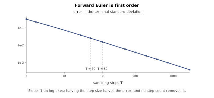
This is the forward Euler method applied to the ordinary differential equation $\mathrm{d}x/\mathrm{d}t = f_\theta(x, t)$, integrated backwards in time; the minus sign is the negative time step, and $1/T$ is its magnitude. Sampling a diffusion model is numerical integration of a learned vector field, and every question about samplers — how many steps, what step sizes, which solver — is a question about numerical integration that the field of numerical analysis had already answered before anyone applied it here.

The step size is why $T$ cannot be one. If the network’s prediction were constant along the trajectory, a single step of size $1$ would land exactly on a data point and diffusion would collapse into a GAN. It is not constant: the predicted velocity is a function of position, and a large step accumulates the error of pretending otherwise. A commonly used value is $T = 50$, and $T = 30$ is often tolerable — meaning that a diffusion model costs thirty to fifty network evaluations per sample against a GAN’s one. That is the price of the stable objective, and Section 15.13 is about trying to get it back.

There is a check worth doing here, because the claim that this procedure produces samples from $p_{\text{data}}$ is not obvious and the lecture asserts it without argument. Take $p_{\text{noise}} = \mathcal{N}(0, 1)$ and $p_{\text{data}} = \mathcal{N}(\mu, \sigma^2)$ in one dimension. Everything is then jointly Gaussian, and the velocity field a perfectly trained network would learn — the conditional expectation $u(x_t, t) = \mathbb{E}[v \mid x_t]$, derived in the next section — is available in closed form:

$$u(x_t, t) = -\mu + \frac{t - (1-t)\sigma^2}{(1-t)^2\sigma^2 + t^2}\,\big(x_t - (1-t)\mu\big). \tag{15.11}$$

Because this is linear in $x_t$, the ODE it defines maps Gaussians to Gaussians, and the mean and variance of the solution can be propagated by integrating two scalar equations. The marginal law of $x_t$ under Equation 15.8 is separately known: it is $\mathcal{N}\big((1-t)\mu,\; (1-t)^2\sigma^2 + t^2\big)$. These are two independent routes to the same quantity, and the chapter’s figure script integrates the first and compares it against the second at every $t$, agreeing to nine decimal places and landing on $\mathcal{N}(\mu, \sigma^2)$ at $t = 0$. The flow really does transport one distribution onto the other.

Figure 15.5: Discretisation error against the number of sampling steps, for the Gaussian problem of Equation 15.11 where the exact answer is known. Both axes are logarithmic, and the measured error is the discrepancy between the terminal standard deviation produced by Equation 15.10 and the true $\sigma$. The slope is $-1$: forward Euler is a first-order method, so halving the step size halves the error, and there is no step count at which the error vanishes. The two step counts the lecture names are marked. This is why a single-step sampler is not merely inaccurate but structurally wrong — at $T = 1$ the method assumes the velocity field is constant over the entire journey from noise to data, which is precisely the assumption that fails.

15.9 What the network can actually predict

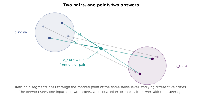
Figure 15.4 left a problem open, and it is the one that determines everything the model can and cannot do. The interpolant $x_t$ does not remember where it came from. A given noisy image is reachable from many different $(x, z)$ pairs, and those pairs carry different velocities, so the training data contains the same input paired with contradictory targets. The network cannot satisfy them all, and squared error decides how it fails: the minimiser of Equation 15.9 is the conditional mean of the target given the input,

$$f^*(x_t, t) = \mathbb{E}\big[\,z - x \;\big|\; x_t\,\big], \tag{15.12}$$

an average over every clean image and every noise sample that could have produced this particular $x_t$. The network is not learning to denoise a specific image. It is learning, at each point of image space and each noise level, the average direction of all the trajectories passing through.

The consequences are cleanest at the two ends. At $t = 0$ there is no ambiguity at all — $x_t$ is the clean image — so the expectation collapses to $\mathbb{E}[z] - x$, the vector from the data point to the mean of the noise distribution, and the problem is trivial. At $t = 1$ the ambiguity is total, since $x_t$ is pure noise and carries no information about which image it will become, so the expectation is $z - \mathbb{E}[x]$: the model can do nothing but point away from the mean image of the entire dataset. Both extremes are easy for the same reason, that neither requires the network to know anything about the data beyond one global statistic.

Everything interesting happens in between, and it is worth being concrete about what the intermediate prediction looks like, because it explains the characteristic behaviour of these models. Rearranging Equation 15.8 gives the clean sample implied by a velocity, $\hat{x} = x_t - t\,f_\theta(x_t, t)$, so the network’s output at any noise level can be read as a guess at the final image. Under Equation 15.12 that guess is $\mathbb{E}[x \mid x_t]$ — an average of every image consistent with the current noisy state. At high noise that average is over almost the whole dataset and is correspondingly featureless; as $t$ falls the set of consistent images narrows and the average sharpens. This is why the intermediate states of a sampling run look the way they do, blurry and global early and detailed late, and it is the same mode-covering blur that ruined the variational autoencoder in the previous chapter. The difference is that here it appears only inside a single step, and the next step is taken from a point where the ambiguity is smaller.

Figure 15.6: What ambiguity costs, on a one-dimensional two-mode dataset where every quantity is closed form. The left panel plots the implied clean prediction $\mathbb{E}[x \mid x_t]$ against the noisy value, at three noise levels: at low noise the curve is a sharp step that commits to whichever mode is nearer, and at high noise it is nearly flat at the dataset mean, meaning the network is producing an average of both modes rather than either one. The right panel measures difficulty as the amount by which the optimal predictor beats the best affine predictor of the same target — that is, how much the network must know about the data beyond its first two moments. This is not the irreducible loss, which stays positive at both ends because the target still contains unobserved noise there; it is the quantity that genuinely vanishes at $t = 0$ and $t = 1$, since the conditional mean is affine at both. The generator asserts both endpoint values are zero. The peak sits nearer $t = 0.3$ than the exact centre, so the logit-normal schedule drawn over it is a rough match to the difficulty rather than a derived one. Both curves are rescaled to their own maximum, because only their shapes are being compared.

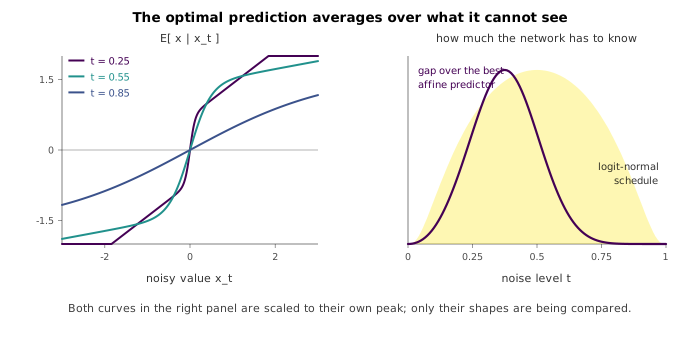
Sampling $t \sim \mathrm{Uniform}(0,1)$ therefore spends equal training effort on noise levels that differ enormously in difficulty. The standard correction is to sample $t$ from a distribution concentrated in the middle, most commonly by drawing a Gaussian variable and squashing it through a sigmoid — logit-normal sampling, used in Stable Diffusion 3 among others. Nothing about the model changes; only the frequency with which each noise level appears in a batch.

The schedule is also where resolution enters, and this is the point at which the clean formulation stops being resolution-agnostic. Adding Gaussian noise of a fixed magnitude destroys much less information in a high-resolution image than in a low-resolution one, because neighbouring pixels in a high-resolution image are strongly correlated and the redundancy survives corruption that would erase an equivalent low-resolution image. A noise level that makes an image genuinely uninformative at $64 \times 64$ leaves a $1024 \times 1024$ image still legible, so the schedule has to be shifted towards higher noise as resolution grows. A diffusion model trained at one resolution does not transfer to another by changing the input size alone, and the beautiful formulation of Section 15.7 turns out to need a resolution-dependent knob before it works on large images.

15.10 Conditioning, and buying obedience with a second forward pass

Unconditional generation is a curiosity. What people want from these models is control: an image of a specific thing, described in words. Rectified flow accommodates conditioning with almost no machinery — the dataset becomes pairs $(x, y)$, the network takes $y$ as an extra input, and both Equation 15.9 and Equation 15.10 are otherwise unchanged. Geometrically the model is now learning a velocity field that points towards $p_{\text{data}}(x \mid y)$, a sub-region of the data distribution, rather than towards all of it.

Trained this way, the model tends to underuse the condition. It learns to produce plausible images and treats the prompt as a suggestion, which is a rational response to an objective in which ignoring $y$ costs only a little loss on most examples. There is no term anywhere in Equation 15.9 that specifically rewards agreement with the condition, so obedience has to be bought at sampling time.

Classifier-free guidance buys it with a change to training that takes one line. On each iteration, flip a coin; if it comes up heads — with probability around one half — replace $y$ with a designated null token before feeding it to the network. The same set of weights now learns two velocity fields at once: $v^\emptyset = f_\theta(x_t, y_\emptyset, t)$, which is the unconditional field pointing towards $p_{\text{data}}(x)$, and $v^y = f_\theta(x_t, y, t)$, which points towards $p_{\text{data}}(x \mid y)$.

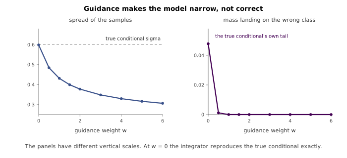
Having both, the difference between them is the part of the velocity that is due to the condition, and it can be amplified. Guided sampling evaluates the network twice and steps along an extrapolation:

$$v^{\mathrm{cfg}} = (1 + w)\, v^{y} - w\, v^{\emptyset} = v^{\emptyset} + (1 + w)\big(v^{y} - v^{\emptyset}\big). \tag{15.13}$$

At $w = 0$ this is the ordinary conditional field. At $w > 0$ the step points further towards the conditional distribution than the model’s own conditional prediction does — past it, in fact, which is why this is extrapolation rather than interpolation and why it is not the same as simply trusting the conditional model. Typical values in deployed systems are between $3$ and $8$.

Figure 15.7: The trade guidance makes, computed by integrating Equation 15.13 on a two-class one-dimensional problem where the exact conditional and unconditional fields are both available in closed form. As the guidance weight rises, the fraction of samples that land closer to the wrong class’s mean falls towards zero — the model obeys the condition — while the standard deviation of the samples within the correct class falls well below the true conditional standard deviation, marked. Guidance does not make the model correct: it makes it narrow. Past a certain weight the samples are cleaner, more prototypical examples of the requested class and a worse sample of the distribution the class actually has, which is the reported behaviour of over-guided text-to-image models — saturated, stereotyped, and short on variety.

The name is a historical accident worth explaining only because the literature is full of it. The earlier technique, classifier guidance, trained a separate classifier $p(y \mid x_t)$ on noisy images and pushed each sampling step along $\nabla_{x} \log p(y \mid x)$, in effect running an adversarial attack on that classifier at every step. Classifier-free guidance obtains the same effect without the second model, and inherited a name that describes what it does not contain.

The cost is arithmetic. Every sampling step now requires two network evaluations instead of one, so guidance doubles the cost of generation on top of the thirty-to-fifty-fold cost the iterative sampler already carries. Against a GAN’s single forward pass, a guided fifty-step diffusion sampler is one hundred network evaluations per image.

15.11 Diffusing somewhere cheaper

A hundred forward passes is survivable if each pass is cheap and ruinous if it is not, and on raw pixels it is not. The claim that diffusion models are the dominant approach to image generation is, strictly, false: what dominates is latent diffusion, which runs the entire construction of the last four sections somewhere other than pixel space.

The pipeline has two stages that are trained separately. First, an encoder and decoder are trained to compress images into a latent representation, downsampling by a factor $D$ spatially while widening the channel dimension to $C$; a common setting is $D = 8$ and $C = 16$, so a $256 \times 256 \times 3$ image becomes a $32 \times 32 \times 16$ latent. Then the encoder is frozen, and a diffusion model is trained on the latents exactly as before: encode an image, interpolate the latent towards noise by Equation 15.8, regress on the velocity. No gradient flows back into the encoder. At sampling time the process runs in reverse — noise in latent space, fifty guided Euler steps, one call to the decoder at the end to turn the clean latent into pixels.

Figure 15.8: The two-stage pipeline and where each network’s gradients stop. The autoencoder is trained first and then frozen; the diffusion model never sees a pixel, and the decoder is invoked exactly once per sample rather than once per step. The token counts along the bottom are for the configuration a current text-to-image model uses, and the $64\times$ reduction they show is the whole reason the pipeline has this shape.

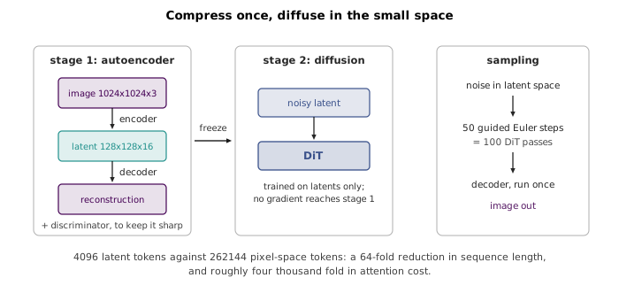
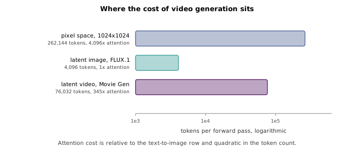
The saving is not subtle. An $8 \times 8$ spatial downsampling removes a factor of $64$ from the number of positions the diffusion network must process, and the transformer that processes them pays attention costs quadratic in that number, so the same architecture costs roughly four thousand times less per forward pass on latents than on pixels. Multiply that by the hundred passes a guided sampler takes and the difference is between a model that can be trained and one that cannot.

What makes the second stage legitimate is that the compression is chosen to be perceptual rather than semantic. The encoder is asked to throw away exactly the high-frequency detail that a reconstruction loss cannot see anyway, leaving the structure that matters, so the diffusion model spends its capacity on content rather than on texture that the decoder can reproduce unaided.

Which raises the question of what the autoencoder is. It is a variational autoencoder — the architecture of the previous chapter, trained with the ELBO of Section 14.12 but with the prior term’s weight turned far down, since nobody intends to sample from this latent space directly and the only thing wanted from the KL term is that the latents not drift to arbitrary scale. But a variational autoencoder’s decoder is blurry, and here the decoder’s output is the final image: whatever it cannot reconstruct, the whole pipeline cannot generate, however good the diffusion model above it.

The fix is the previous section of this chapter. Add a discriminator on the decoder’s output and train the autoencoder adversarially alongside its reconstruction loss, which restores the high-frequency detail that the Gaussian likelihood averages away. Note where the GAN has ended up: not as the generative model, where it was uncontrollable, but as a perceptual loss on an autoencoder, where the thing it is asked to do is local and the training is stabilised by the reconstruction term sitting next to it.

So the state of the art is not one of the families in these two chapters. It is a variational autoencoder, trained with an adversarial loss, whose frozen latent space carries a diffusion model, conditioned on the output of a pretrained language model. Every family in this course’s treatment of generative modelling appears in the modern pipeline, doing the one job it does well.

15.12 The backbone, and where the conditioning attaches

The network inside all of this is a plain transformer. Diffusion transformers cut the latent into patches, treat the patches as a sequence, and run standard blocks over them; there is no diffusion-specific architecture, and the U-Nets that earlier diffusion models used have largely been replaced. The one genuine design question is how three quite different inputs — the noisy latent, the scalar timestep, and the conditioning signal — get into a stack that takes a sequence.

They get in by two different routes, chosen to match their shapes. The timestep is a single scalar shared by every position, so it is injected by modulation: a small network maps $t$ to a per-channel scale and shift that rescale the normalised activations inside each block, which is the same adaptive-normalisation mechanism Equation 15.7 used in StyleGAN, applied here to a different quantity. The conditioning signal is itself a sequence — a text prompt is a variable number of embedding vectors — so it is injected by attention, either through cross-attention layers that let image tokens attend to text tokens, or by concatenating both into one sequence and running joint attention over the whole thing. The DiT paper compares these choices directly and finds adaptive normalisation the strongest for the timestep.

For text-to-image, the text embeddings come from a pretrained, frozen encoder — T5, CLIP, or both — so the language understanding is inherited rather than learned. The full path for a current open-weights model, FLUX.1, is: prompt through the frozen text encoders; a $1024 \times 1024$ target image corresponding to a $128 \times 128 \times 16$ latent; a $2 \times 2$ patchify on top of the autoencoder’s downsampling, giving a $64 \times 64$ grid, which is $4{,}096$ image tokens; a twelve-billion-parameter transformer run once per sampling step; and the decoder run once at the end. The deck states this token count as $1{,}024$, which does not follow from the $64 \times 64$ grid on the same line — the sequence a model in this configuration processes is $4{,}096$ tokens, and that is the number the video comparison below is built on.

15.13 Video, and the bill for many steps

Text-to-video changes one thing in the diagram and it is not the architecture. The latent acquires a time axis, so it is $t \times h \times w \times c$ instead of $h \times w \times c$; the autoencoder becomes spatio-temporal, downsampling in time as well as space; and everything else — the DiT, the frozen text encoder, guided Euler sampling — is unchanged. Meta’s Movie Gen uses $8 \times 8 \times 8$ downsampling and a thirty-billion-parameter transformer to produce a $257$-frame $1024 \times 576$ video from a $33 \times 128 \times 72 \times 16$ latent.

The difficulty is entirely in the sequence length. A $1 \times 2 \times 2$ patchify over that latent yields about $76{,}000$ tokens against a text-to-image model’s $4{,}096$ — around nineteen times as many, and since attention is quadratic, roughly three hundred and forty times the attention cost per forward pass. This is why video models are expensive in a way that does not follow from their parameter counts, and why the entire field’s progress over the eighteen months to mid-2025 reads as a sequence-length engineering problem more than a modelling one.

Figure 15.9: Where the cost sits, on a logarithmic axis because the quantities span four orders of magnitude. Bars show the sequence length a transformer processes under three configurations — pixel space at the target resolution, the latent used by a current text-to-image model, and the latent used by a current text-to-video model — with the quadratic attention cost of each shown relative to the text-to-image case. Latent diffusion buys back four orders of magnitude of attention cost; adding a time axis gives most of that back. The numbers are computed from the downsampling and patchify factors the respective models report, and the axis is logarithmic, so equal bar lengths represent equal ratios rather than equal differences.

That leaves the other cost, the one Section 15.8 introduced and every section since has multiplied: a sample requires tens of sequential forward passes through a very large model, and guidance doubles them. Distillation is the family of methods aimed at this. The shared idea is to train a student that reproduces what the many-step sampler produces in far fewer steps — sometimes one — by supervising it against the teacher’s trajectory or its endpoint rather than against the data. All of them trade sample quality for step count, and the research question is how little quality has to be given up; single-step distillation works and visibly costs something. This is an area moving fast enough that any specific method named here would date quickly, which is a reasonable summary of where inference-time efficiency in generative modelling currently stands.

15.14 One object, several languages

Section 15.7 presented one specific recipe, and the reason the literature is hard to read is that almost every paper presents a different one. The differences are smaller than the notation suggests. Write the training step in its general form: sample $x$ and $z$, sample $t \sim p_t$, and then

$$x_t = a(t)\,x + b(t)\,z, \qquad y_{\text{gt}} = c(t)\,x + d(t)\,z, \tag{15.14}$$

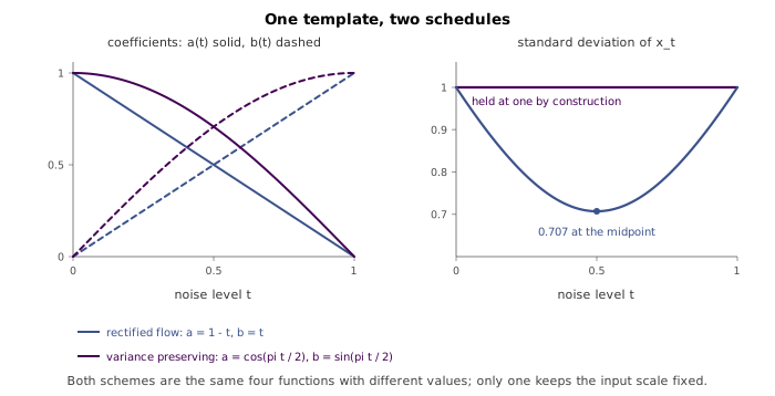
with the loss always $\lVert f_\theta(x_t, t) - y_{\text{gt}} \rVert_2^2$. Four scalar functions of $t$, and every variant is a choice of those four. Rectified flow takes $a = 1-t$, $b = t$, $c = -1$, $d = 1$, the last two being constants, which is why its target is the simple difference $z - x$.

Two other choices are common enough to name. Variance-preserving schemes set $a(t) = \sigma(t)$ and $b(t) = \sqrt{1 - \sigma(t)^2}$, collapsing the two interpolation coefficients into a single noise schedule chosen so that $a^2 + b^2 = 1$; when $x$ and $z$ are independent with unit variance, $x_t$ then has unit variance at every noise level, which keeps the network’s input distribution constant across $t$. Variance-exploding schemes take the opposite tack, $a(t) = 1$ and $b(t) = \sigma(t)$, leaving the data untouched and adding noise of growing magnitude on top, which requires $\sigma(1)$ to be large enough to drown the signal entirely.

Figure 15.10: The two most common interpolation schemes, and the property one of them is named for. The left panel plots the coefficients $a(t)$ and $b(t)$ against noise level: rectified flow’s are straight lines, while the variance-preserving pair traces a quarter circle. The right panel plots the resulting standard deviation of $x_t$ for unit-variance data and noise. Variance preservation is exactly the flat line — the network sees inputs of the same scale at every noise level — while the linear interpolation sags to $1/\sqrt{2}$ in the middle, so a rectified-flow network must cope with an input whose magnitude varies by thirty per cent over the range of $t$ it is trained on.

The target functions $c$ and $d$ have names too. Setting $c = 1, d = 0$ is $x$-prediction, asking the network for the clean image; $c = 0, d = 1$ is $\epsilon$-prediction, asking for the noise that was added, which is what the original denoising diffusion papers used; and $c = b(t), d = -a(t)$ is $v$-prediction. These are not different models. Given $x_t$ and $t$, any one of the three determines the other two by Equation 15.14, so a network trained on one target can be read as predicting any of them. What differs is the implied weighting of the loss across noise levels, since predicting the noise at low $t$ is a differently scaled problem from predicting the image there, and that weighting matters in practice even though the parameterisations are formally equivalent.

Choosing four functions of $t$ by intuition is hopeless, which is why the field reaches for mathematics, and there are three distinct frameworks that supply it. The first treats diffusion as a latent variable model: the noisy versions $x_1, \ldots, x_T$ of a clean image are unobserved variables with a known forward process, the network approximates the reverse process, and training maximises a variational lower bound derived exactly as in Section 14.12. This is the DDPM formulation, and under it a diffusion model is a very deep variational autoencoder whose encoder has no parameters.

The second treats diffusion as score estimation. For any density $p$, its score is the gradient of its log,

$$s(x) = \nabla_x \log p(x), \tag{15.15}$$

a vector field pointing towards regions of higher probability. The claim is that a diffusion network learns not one score but a family of them, one for each noise level, for the sequence of increasingly smoothed distributions $p_t$. That claim is checkable rather than atmospheric, because the score and the velocity are related by an exact affine identity. Conditioned on $x$, the interpolant is Gaussian with mean $(1-t)x$ and standard deviation $t$, and averaging its score over the posterior gives $\nabla \log p_t(x_t) = -\mathbb{E}[z \mid x_t]/t$; substituting the optimal velocity from Equation 15.12 yields

$$\nabla_{x_t} \log p_t(x_t) = -\frac{x_t + (1-t)\, f^*(x_t, t)}{t}. \tag{15.16}$$

The chapter’s figure script checks this by computing the left-hand side directly, differentiating the closed-form marginal density of the Gaussian problem in Equation 15.11, and comparing it against the right-hand side built from Equation 15.11 itself. They agree to twelve decimal places across the range of $t$. The velocity network and the score network are the same network in different clothes.

The third treats diffusion as solving a stochastic differential equation, $\mathrm{d}x = f(x, t)\,\mathrm{d}t + g(t)\,\mathrm{d}w$, which describes the noising process as a continuous-time random walk and generation as its time reversal. Its practical payoff is that sampling becomes a problem in numerical integration with a literature attached, and Equation 15.10 is revealed as the crudest method in that literature — forward Euler on the deterministic reduction of the equation. Better integrators exist, which is where much of the recent progress on few-step sampling comes from. Sander Dieleman’s survey of these perspectives counts eight rather than three and is the best entry point to the area.

15.15 Autoregression comes back

The previous chapter dismissed autoregressive models for images on a single ground: sampling costs one network pass per subpixel, which is millions of sequential passes for a real image. That argument is about pixels, not about autoregression, and Section 15.11 showed how to stop working in pixels.

The construction is the same two-stage pipeline with a different second stage. Train an encoder and decoder that map images to a grid of discrete latents — integers drawn from a learned codebook, as in VQ-VAE — and then train an autoregressive transformer over the resulting sequence of tokens, exactly as a language model is trained over text. Generation samples tokens one at a time from the transformer and hands the completed grid to the decoder. A $32 \times 32$ latent grid is $1{,}024$ sequential steps rather than three million, which is expensive but no longer absurd, and the model recovers the exact likelihood that the diffusion route gives up.

The two modern recipes are therefore the same shape — compress, model the compressed representation, decode — and differ only in what models the middle. That is a more useful summary of the field than a list of five families, and it is why both chapters were necessary before either recipe could be stated.

15.16 What each family bought

The previous chapter’s ledger can now be completed. Each row is a consequence of one design decision rather than of architecture, and no column dominates.

	Autoregressive	Variational autoencoder	GAN	Diffusion
Density $p(x)$	exact	lower bound	none	bound, via Section 15.14
Latent code	none	explicit	implicit, no encoder	same shape as the data
Passes per sample	one per token	one	one	30–100
Training signal	likelihood	likelihood	a second network	regression on noise
Characteristic failure	slow sampling	blur	mode collapse	slow sampling

The pattern across the row for training signal is the one worth carrying away. Maximum likelihood is stable and mode-covering, and its price is paid in blur. Adversarial training is mode-seeking and sharp, and its price is paid in stability. Diffusion’s contribution was to notice that these are not the only two options: a plain regression loss, applied to a problem decomposed into steps small enough that each one has a well-defined answer, is stable like the first and sharp like the second, and pays instead in sampling time — the one currency that hardware and distillation research can actually work on.

What the field settled on is not a winner but an assembly. A modern text-to-image system contains a variational autoencoder for compression, a discriminator to keep its decoder sharp, a diffusion transformer in the latent space, and a frozen language model for the conditioning; the autoregressive alternative swaps the third component and keeps the rest. Every family in these two chapters is in the pipeline, doing the job that its particular trade-off makes it good at.