12  Large-Scale Distributed Training

Lecture 11

Based on Lecture 11 of CS231n, Stanford University, Spring 2025.

12.1 Twenty-five thousand computers, one model

Every chapter up to this one has described a computation that fits on a single device. A network is a function, the gradient of its loss is computed by backpropagation, and an optimizer applies that gradient to the weights. Nothing in that account mentions where the weights live, because for the first decade of the field the answer never had to be interesting: they lived in the memory of one GPU, and if they did not fit you trained a smaller model.

That assumption has quietly become false for every model at the frontier, and undoing it is not a matter of engineering hygiene. The gradient of a loss is defined over a batch; if the batch is spread across sixteen thousand devices, then computing that gradient is a communication problem before it is an arithmetic one, and the algorithms in this chapter exist because the communication is what runs out first.

The running example throughout is Llama 3 405B, and the choice is made on grounds of disclosure rather than quality. GPT-4 marked the point at which the industry stopped publishing: its technical report states outright that it “contains no further details about the architecture (including model size), hardware, training compute, dataset construction, training method, or similar,” and essentially every frontier lab has followed. Meta’s Llama 3 paper is the exception that makes a chapter like this possible — it describes the cluster, the parallelism configuration, the utilisation achieved, and even the failure rate.

Four numbers set the problem. The model has 405 billion parameters. It was pre-trained on 15.6 trillion text tokens. The pre-training compute budget was $3.8 \times 10^{25}$ floating-point operations. And it ran on up to 16,384 H100 GPUs, drawn from a cluster of about 24,000.

Those numbers are not independent, and the relation between them is the single most useful piece of arithmetic in the chapter. For a dense transformer, a forward pass costs roughly two FLOPs per parameter per token — one multiply and one add for each weight the token passes through — and the backward pass costs about twice the forward. The total is

$$C \approx 6 N D \tag{12.1}$$

where $N$ is the parameter count and $D$ the number of training tokens. Substituting Llama 3’s figures gives $6 \times 4.05 \times 10^{11} \times 1.56 \times 10^{13} = 3.79 \times 10^{25}$, which is the published budget to two significant figures. The rule is crude — it ignores attention’s quadratic term, normalisation, and the embedding layers — and it is accurate enough that it is how training runs are actually planned.

Equation 12.1 also says what the rest of this chapter is for. Divide the budget by what the hardware can deliver: 16,384 GPUs sustaining 400 TFLOP/s each is $6.6 \times 10^{18}$ FLOP/s, so $3.8 \times 10^{25}$ operations take about 5.8 million seconds, or roughly two months of wall-clock time at full utilisation. That figure is consistent with the paper, which reports statistics over a 54-day snapshot of pre-training. The entire difficulty is in the phrase at full utilisation, because the naive way of using sixteen thousand GPUs achieves a small fraction of it, and every technique below is a way of clawing some of that fraction back.

It is worth registering what a run of that length means physically before treating the cluster as an abstraction. Over those 54 days Meta recorded 466 job interruptions, of which 419 were unexpected; about 78% were traced to hardware, and GPU failures alone accounted for 58.7% of them. That is roughly eight unplanned failures a day on a machine that has to behave as one computer for two months. Only three of them required manual intervention. The rest is the price of building something out of twenty-five thousand physical objects.

12.2 Inside one GPU

A GPU is not a fast CPU. It is a device whose entire design is organised around doing the same arithmetic to a great many operands at once, and the two facts that matter for training — the memory hierarchy and the tensor cores — both follow from that.

Take the H100, which is the workhorse of the current generation. At the coarsest level it is a die of compute surrounded by 80 GB of high-bandwidth memory, connected by a bus that moves about 3,352 GB/s. That number sounds enormous until it is compared against the compute it feeds. Inside the compute die sits 50 MB of L2 cache, three orders of magnitude smaller than the HBM but far closer to the arithmetic units, and beneath that, 132 streaming multiprocessors, each with 256 KB of L1 cache and 256 KB of registers.

The pattern is the point, and it recurs at every scale in this chapter: memory that is larger is further away, and memory that is closer is faster and smaller. Writing a fast kernel is largely the discipline of staging data down that hierarchy and reusing it while it is close, and — as Section 12.3 shows — writing a fast distributed training job is the same discipline applied to a hierarchy that extends past the boundary of the chip.

Figure 12.1: The four levels of the hierarchy for which the Llama 3 cluster publishes a bandwidth, with the memory reachable at each printed at the right. Every step outward multiplies the capacity available and divides the rate at which it can be reached. The cross-pod figure is derived rather than published: the paper gives a 1:7 oversubscription ratio at the aggregation layer, applied here to the pod bandwidth. Drawn for this project from the paper’s network description.

A detail of manufacturing is worth a sentence because it explains a number that otherwise looks arbitrary. The H100 die physically contains 144 streaming multiprocessors, but only 132 are enabled. Chips of this transistor count never come off the line perfect, so vendors bin them: the design targets 144, the product promises 132, and the dies with a handful of defective units are sold rather than discarded. Nearly every published core count in this field is a yield-adjusted floor, not a description of the silicon.

12.2.1 Where the throughput actually comes from

Zoom into one streaming multiprocessor and there are two kinds of arithmetic unit, with wildly different capabilities.

The first is a bank of 128 FP32 cores. Each computes $ax + b$ for scalars $a$, $x$, $b$ in one clock cycle — a fused multiply-add, counted as two floating-point operations. One SM running its FP32 cores therefore retires $128 \times 2 = 256$ FLOP per cycle.

The second is four tensor cores, and the name undersells them: they are matrix cores. Each performs one small matrix multiply-accumulate per clock, on the H100 taking a $16 \times 4$ input against a $4 \times 8$ input and adding a $16 \times 8$ accumulator. Counting a multiply and an add for each of the $16 \times 4 \times 8$ scalar products gives $1{,}024$ FLOP per tensor core per cycle, so four of them retire $4{,}096$ FLOP per cycle:

$$\underbrace{16 \times 4 \times 8 \times 2}_{1024\ \text{FLOP per tensor core}} \times 4 = 4096 \quad\text{versus}\quad \underbrace{128 \times 2}_{\text{FP32 cores}} = 256 \tag{12.2}$$

A factor of sixteen, on the same silicon, in the same cycle. It is not an exaggeration to say that the tensor cores are the device and the FP32 cores are what runs when you have made a mistake.

The catch is precision. Tensor cores operate in mixed precision: the inputs arrive as 16-bit floats, the multiplications happen at 16 bits, and the accumulation is carried at 32 bits so that summing many products does not destroy the result. This is why a model that is not cast to a 16-bit dtype silently runs on the FP32 path instead — and why the symptom is not an error but training that is inexplicably twenty times slower than expected. Mixed precision is not an optimisation applied to a working training script; it is the condition under which the hardware is being used at all.

12.2.2 A thousandfold, with an asterisk

The generational numbers make the last decade legible. The K40 of 2013 delivered 5 TFLOP/s of FP32. The P100 reached 10.6. The V100 of 2017 was the first device with tensor cores and offered 125 TFLOP/s on them against 15.7 in FP32. The A100 followed with 312 and 19.5, the H100 with 989 and 67, and the B200 with roughly 5,000 and 83.3.

The headline conclusion drawn from that series — a thousandfold speedup in twelve years — deserves an asterisk, because it compares the B200’s tensor cores against the K40’s FP32 cores. Measured like against like, general-purpose floating-point throughput grew by about seventeen times, from 5 to 83.3 TFLOP/s, which is roughly what Moore’s law would predict over that span. The remaining factor of sixty came from two decisions rather than from transistor density: spending die area on units that do nothing but matrix multiply-accumulate, and halving the precision of the operands.

That is a more interesting fact than the headline, because it says the speedup was bought by specialising — by building hardware that is fast only for a narrow computation and then reorganising deep learning to consist of that computation. Architectures that reduce to large dense matrix multiplies ride the curve; architectures that do not are stranded on the seventeenfold line. The dominance of the transformer, which is very nearly nothing but matrix multiplies, is not unrelated.

12.3 From a chip to a cluster

Set the single device aside and consider the machine that Llama 3 was actually trained on, because the shape of the parallelism strategies in the second half of this chapter is dictated almost entirely by its wiring.

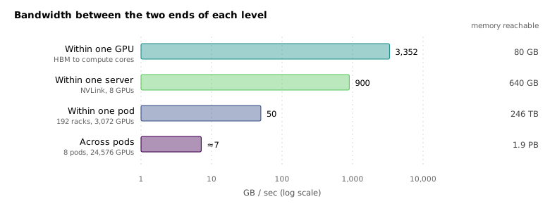
Inside one H100, memory reaches the cores at 3,352 GB/s. Eight of those GPUs sit in one server, connected to each other by NVLink at about 900 GB/s — roughly a quarter of on-device bandwidth, and the first cliff. Two servers make a rack of 16 GPUs. 192 racks are joined by cluster switches into a pod of 3,072 GPUs with full bisection bandwidth, at which point any GPU can reach any other at about 50 GB/s. That is another factor of eighteen down. Eight pods make the full cluster of 24,576 GPUs, and here the network is deliberately oversubscribed at a ratio of 1:7, so cross-pod bandwidth is materially worse than 50 GB/s.

Read as one object, that cluster has 1.875 PB of GPU memory, 415 million FP32 cores, 13 million tensor cores, and a peak of 24.3 EFLOP/s — $2.43 \times 10^{19}$ floating-point operations per second. The productive way to think about it is not as twenty-five thousand computers but as one computer with a four-level memory hierarchy bolted onto the four levels already inside each chip, and with the same rule holding across all eight: further away means larger and slower.

The consequence is the organising principle of everything that follows. A computer does two things — it computes, and it moves bits from one place to another. Compute is what you want; communication is overhead. There are only two ways to reduce the damage that communication does. The first is to hide it, by arranging for bits to be in flight during a stretch of arithmetic that does not need them yet. The second is to place it, by assigning the communication-hungry parts of the algorithm to the links that are fast and the communication-light parts to the links that are slow. Every technique in the remainder of this chapter is one or both of those moves.

Two footnotes on the hardware landscape. NVIDIA is dominant but not alone: Google’s TPUs are in their sixth generation, with the v5p offering 459 TFLOP/s of BF16 per chip and 95 GB of memory, arranged into pods of up to 8,960 chips, and Google’s own frontier models are almost certainly trained on them. The difference is commercial rather than technical — TPUs cannot be bought, only rented. AMD’s MI325X (1,300 TFLOP/s BF16, 256 GB) and AWS’s Trainium2 (667 TFLOP/s BF16, 96 GB, packaged 64 to an UltraServer) have competitive datasheets and much less software gravity behind them. The second footnote is that the interconnect numbers above are the Llama 3 cluster’s specifically; the topology generalises, the exact bandwidths do not.

12.4 Four axes and a budget

The rest of the chapter is about splitting a transformer across that machine, and it helps to know in advance that there are only four places to cut.

A transformer is a stack of $L$ layers, each operating on a tensor of shape $(B, S, D)$ — a minibatch of $B$ sequences, each of $S$ tokens, each token a vector of dimension $D$. That is four indices, and each one is an axis of parallelism with a name:

Axis	Name	Abbrev.
batch $B$	data parallelism	DP
sequence $S$	context parallelism	CP
feature $D$	tensor parallelism	TP
layers $L$	pipeline parallelism	PP

Figure 12.2: The four axes of a transformer’s computation and the parallelism strategy that splits each. A layer’s activations form a $(B, S, D)$ tensor and the model is a stack of $L$ of them; every distributed training scheme in this chapter is a choice of how many ways to cut along each of these four indices. Drawn for this project.

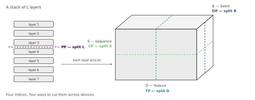
The names are opaque and the underlying idea is not: they are four ways of cutting the same block of computation, and a real training run cuts along all of them at once. What decides how much of each is the memory budget, so it is worth doing that arithmetic now.

Storing a trained model requires one number per parameter. Training one requires four or five. There is the weight itself; the gradient with respect to it; and, for Adam, the first and second moment estimates — one exponentially weighted average of the gradient and one of its square. Some setups additionally keep an exponential moving average of the weights for evaluation. At 16-bit precision each of these is two bytes, so a lower bound is

$$\text{bytes per parameter} = \underbrace{4}_{\text{weight, grad, } m, v} \times \underbrace{2}_{\text{bytes at 16-bit}} = 8 \tag{12.3}$$

A billion parameters therefore occupies 8 GB before a single activation is stored, and an 80 GB H100 is full at around ten billion. Llama 3 405B needs some 3.2 TB by this accounting — forty H100s’ worth of memory to hold the state of a model that has not yet been given any data to process.

This is the wall. Every technique from here on is a response to some part of it: Section 12.5 accepts it and scales the batch instead, Section 12.6 attacks the eight bytes directly, Section 12.8 attacks the activations that Equation 12.3 ignores, and Section 12.10 through Section 12.12 attack the assumption that one layer’s computation has to happen on one device.

12.5 Data parallelism

The easiest axis to cut is the batch, and the reason is one line of algebra.

Training minimises a loss that is an average over the minibatch, and the gradient of an average is the average of the gradients. Write the macro-batch as $MN$ samples $x_{i,j}$, indexed so that $i$ runs over $M$ devices and $j$ over the $N$ samples each device holds. Then

$$\frac{\partial}{\partial W} \left[ \frac{1}{MN} \sum_{i=1}^{M} \sum_{j=1}^{N} L(x_{i,j}, W) \right] = \frac{1}{M} \sum_{i=1}^{M} \underbrace{\frac{1}{N} \sum_{j=1}^{N} \frac{\partial L(x_{i,j}, W)}{\partial W}}_{\text{an ordinary forward–backward on } N \text{ samples}} \tag{12.4}$$

The bracketed inner term is exactly what a single GPU already computes when handed a minibatch of $N$ examples. The outer sum is an average of $M$ such quantities. Linearity lets the summation and the differentiation be reordered at no cost, and the reordering assigns the inner term to a device and the outer term to the network.

The emphasis belongs on at no cost. This is not an approximation of single-device training and not a variant of SGD with different convergence behaviour — it is the same computation, rearranged. Given deterministic arithmetic, $M$ GPUs running Equation 12.4 produce bit-for-bit what one impossibly large GPU would have produced on the macro-batch.

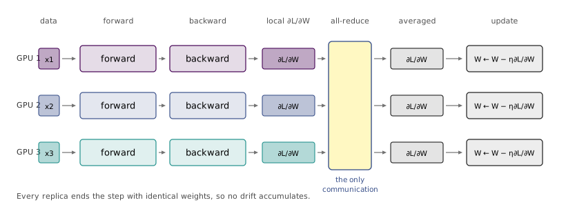
The procedure follows directly. Every GPU holds its own complete copy of the weights, the gradients and the optimizer state. Every GPU loads a different minibatch — accidentally loading the same data on all devices is a real and easily made bug, and it turns an $M$-fold increase in cost into no increase in information. Every GPU runs forward on its own data to a local loss, and backward to a local gradient. Then, and only then, communication: an all-reduce in which each device simultaneously broadcasts its gradient to every other device and accumulates everyone else’s, ending with all $M$ devices holding an identical copy of the averaged gradient. A good implementation does this in time logarithmic in $M$ rather than linear. Each device applies that gradient to its own weights, and because they began the step with identical weights and applied an identical update, they end it with identical weights, and the invariant is restored.

Figure 12.3: Data parallelism across three devices. The forward and backward passes are entirely local — each device sees only its own minibatch and computes only its own local gradient — and the single point of communication is the all-reduce that averages those gradients. After it, every device holds the same gradient and applies the same update, so the replicas never drift apart. Drawn for this project.

12.5.1 Hiding the all-reduce

Written as five sequential steps, this leaves the interconnect idle during the backward pass and the tensor cores idle during the all-reduce. Neither is acceptable, and the fix is the first instance of the hiding move from Section 12.3.

Backpropagation produces gradients one layer at a time, starting from the last layer. The gradient of the final layer is complete and ready to be communicated at a moment when the device still has the entire rest of the backward pass ahead of it. So launch the all-reduce for layer $\ell + 1$ as the backward pass for layer $\ell$ begins, and let the two proceed concurrently. In the steady state the network is always reducing the gradient of the layer above the one the tensor cores are currently differentiating, and if the interconnect can keep up, the last all-reduce completes at almost the same instant as the last local gradient. The optimizer step then runs with no waiting at all.

Whether the interconnect can keep up is a question with no general answer — it depends on the model size, the local batch size, the depth, and the link bandwidth, and the only honest way to find out is to measure the specific configuration. What is general is that none of this scheduling is automatic. Within a single GPU, CUDA overlaps a great deal of memory movement with computation in hardware; across the cluster, nothing does, and the interleaving has to be expressed in software. In PyTorch that software is DistributedDataParallel, which registers hooks on the backward pass and issues the collectives at the right moments, so ordinary single-device training code inherits the overlap without being rewritten.

It is worth naming the alternative that this design rejects. One could let each replica take several optimizer steps independently and reconcile the weights occasionally — asynchronous SGD, which Google used for some early-2010s models before the TPU pods existed. It communicates far less. It is also less stable, harder to reproduce, and harder to debug, and it tends to reach worse solutions, so the field settled on synchronous updates wherever they are affordable. The tradeoff is not permanent: as clusters grow and interconnects fail to keep pace, asynchronous methods may become attractive again for exactly the reason they were abandoned.

12.5.2 The ceiling

Data parallelism scales the batch beautifully and does nothing whatsoever about the model. Every device still holds a full copy of the weights, gradients and optimizer state, so Equation 12.3 applies unchanged and the largest trainable model is capped at around ten billion parameters on an 80 GB device no matter how many devices there are. Adding GPUs buys throughput and buys no capacity.

That is the wrong tradeoff for the models people actually want, and the fix is to notice that the replication is pure waste: $M$ devices are storing $M$ identical copies of the same optimizer state and using each copy once per step.

12.6 Fully sharded data parallelism

Give every weight matrix an owner. Assign each layer’s parameters to exactly one of the $M$ GPUs, and make that GPU responsible for the layer’s gradient and optimizer state as well. Memory for model state now falls by a factor of $M$, because nothing is stored twice. This is fully sharded data parallelism, and the sharding is by layer, not by scalar — $W_i$ throughout means an entire layer’s weight matrix.

Everything else about data parallelism survives. Each GPU still loads its own minibatch, still runs a full forward and backward pass over the whole network on that minibatch, and still ends up contributing to a gradient averaged over the macro-batch. What changes is that a device no longer possesses the weights it needs, so they have to be fetched.

The forward pass becomes a repeated cycle. Before layer 1 can run, the GPU that owns $W_1$ all-gathers it to every other GPU. All devices now hold $W_1$, and all run layer 1 on their own local activations. Immediately afterwards, every device that does not own $W_1$ deletes its copy, returning memory to the sharded state — but keeping the layer-1 activations, which are needed for backward. Then the owner of $W_2$ broadcasts, and so on to the end of the network. The same hiding move applies: while layer $i$ computes, the weights for layer $i+1$ are already in flight, so in the steady state the gather for the next layer is free.

The backward pass has three things to overlap rather than two, and the extra one is the return trip for gradients. For each layer, in reverse order: the owner gathers the weights out to everyone; every device computes its local gradient for that layer; and every device sends that local gradient back to the owner, which sums them. This last collective is a reduce-scatter rather than an all-reduce — the reduction lands on one device instead of on all of them, which is both cheaper and exactly what is wanted, since only the owner will apply the update. Once the owner has the full macro-batch gradient it takes the optimizer step for that layer alone. Notably, it does not then have to broadcast the updated weights, because the next forward pass will gather them anyway.

Figure 12.4: The steady state of an FSDP backward pass. Three things happen concurrently on three different resources: the tensor cores compute the backward pass for layer $\ell$, the interconnect gathers the weights for layer $\ell - 1$, and the reduce-scatter plus optimizer step for layer $\ell + 1$ completes. Communication is only free while all three stay in step. Drawn for this project.

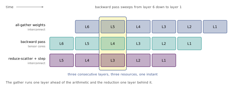
In the steady state of a deep network, then, three consecutive layers are in play at once: layer $\ell + 1$ is having its gradients reduced and its weights updated, layer $\ell$ is being differentiated, and layer $\ell - 1$ is having its weights prefetched. Add asynchronous data loading on the host CPUs and the next batch is ready before the current one finishes. The whole system is a machine for keeping the tensor cores fed.

One optimisation is worth stating because it generalises. At the end of the forward pass every device is holding the last layer’s weights, and the very next thing that happens is the backward pass for the last layer, which needs those same weights. So do not delete them. It is a small saving on its own, and it is an instance of the rule that governs all of these schemes: a gather you can skip is worth more than a gather you can hide, because hiding it still consumes bandwidth that something else wanted.

The cost of FSDP is that it communicates far more than plain data parallelism. Over one forward-backward pass, the weights cross the network once during forward and again during backward, and the gradients cross once more — roughly three times the model size, against one for plain data parallelism, which moves only the gradients. That ratio is the whole reason the next section exists.

12.7 Hybrid sharding

FSDP has one axis, and a cluster has a hierarchy. Putting a single sharding group across the full cluster means paying the three-model-sizes communication cost over the slowest links in the machine, which is precisely backwards: the most communication-hungry strategy has been assigned the worst wires.

Hybrid sharded data parallelism fixes this by arranging the GPUs in a two-dimensional grid. Along one axis, groups of $K$ GPUs each run ordinary FSDP among themselves, with the model sharded $K$ ways inside the group. Along the other axis, $M$ such groups run ordinary data parallelism against each other — each group holds a complete copy of the model, processes its own share of the macro-batch, and at the end of the backward pass the groups all-reduce their gradients with one another.

Figure 12.5: Hybrid sharding as a two-dimensional grid. Within a group the model is sharded and the traffic is roughly three model sizes per step, so groups are made to coincide with the fast domain — the eight GPUs of a server, joined by NVLink. Across groups the model is replicated and only gradients move, one model size per step, which is what the slower inter-server links can afford. Drawn for this project.

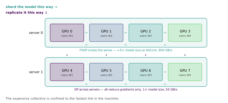
The point of the arrangement is that the two axes have different appetites, and the cluster has different links. Sharding costs three model sizes of traffic per step; replication costs one. So make the sharding groups coincide with the fast domain — the eight GPUs inside a server, joined by NVLink at 900 GB/s — and let the replication axis span servers, racks and pods, where bandwidth is an order of magnitude worse but only a third as much has to cross.

This is the first algorithm in the chapter designed against a specific network topology rather than against an abstract collection of devices, and it will not be the last. It is also the second move from Section 12.3 in its purest form: not hiding communication, but placing it.

12.7.1 A recipe, and where it stops

The three schemes so far compose into a practical sequence, and it is worth writing down because most readers will never need anything past it.

Start with plain data parallelism. It works well up to roughly 128 GPUs and models of around a billion parameters, and the local batch size should be set as large as GPU memory allows — that is almost always the right call, since it maximises the arithmetic done per unit of communication. Past a billion parameters the model state stops fitting comfortably and it is time for FSDP, which buys an order of magnitude of model size and scales to several hundred devices. Somewhere between 256 and 512 GPUs, depending on the cluster, FSDP’s three-model-sizes cost outgrows the interconnect, and the sharding group should be capped and replicated instead — that is, HSDP. Together these reach models of tens of billions of parameters on about a thousand GPUs.

Beyond that — more than a thousand GPUs, more than fifty billion parameters, or sequences longer than ten thousand tokens — the batch axis is exhausted and the remaining three axes of Figure 12.2 have to be brought in. Before they are, there is a second memory problem that none of the above touches, and a metric that decides all the tradeoffs.

12.8 Activations, and paying compute to store fewer of them

Sharding solves the model-state problem completely. A hundred-billion-parameter model needs 800 GB by Equation 12.3, and split across eighty GPUs that is 10 GB each — comfortable. The memory then fills up anyway, because of the thing Equation 12.3 does not count.

Backpropagation requires the activations. Every layer’s backward pass needs the input it saw during the forward pass in order to compute the gradient, so the forward pass cannot discard as it goes; it accumulates. And unlike the model state, activation memory scales with the batch and the sequence length as well as with the depth.

The arithmetic for Llama 3 405B is bracing. It has 126 layers and a model dimension of 16,384, and the first pre-training stage used sequences of 8,192 tokens. Storing one tensor per layer for a single sequence at 16-bit precision costs

$$126 \times 8192 \times 16384 \times 2\ \text{bytes} \approx 33.8\ \text{GB} \tag{12.5}$$

That is 42% of an 80 GB H100 for one sequence, and it is an underestimate by a wide margin, because a transformer block stores considerably more than one tensor — the attention projections, the softmax output, the two MLP intermediates, and the normalisation inputs are all live. There is no batch size that makes this work.

The escape is that activations are not data; they are recomputable. Every one of them is a deterministic function of the input, so any activation that has been thrown away can be reconstructed by running the forward pass again. This trades compute for memory, and compute is the thing the tensor cores have in abundance.

Model a network as $N$ layers, each of which is two functions: a forward $A_{i+1} = F_i^{\rightarrow}(A_i)$ and a backward $G_i = F_i^{\leftarrow}(A_i, G_{i+1})$, each costing one unit of compute and one unit of memory. Ordinary training runs $N$ forward steps, holding on to all $N$ activations, then $N$ backward steps: $O(N)$ compute and $O(N)$ memory.

At the other extreme, keep nothing but the input. The forward pass runs and discards as it goes. The backward pass for the last layer is fine, but the backward pass for layer $i$ needs $A_i$, which is gone, so it is regenerated by rerunning layers $1$ through $i-1$. Summing that over all $i$ gives $N + \sum_{i=1}^{N} i = O(N^2)$ compute for $O(1)$ memory. The memory problem is solved and replaced by a compute problem that is worse, since $N$ is in the hundreds.

The useful regime is between them. Keep $C$ checkpoints, spaced $N/C$ layers apart, and recompute from the nearest one whenever a backward step needs an activation it does not have. Each such recomputation walks at most a segment, so

$$\text{compute} = O\!\left(\frac{N^2}{C}\right), \qquad \text{memory} = O(C) \tag{12.6}$$

There is no interior optimum here — Equation 12.6 is a pure exchange rate, and $C$ should be pushed as high as the memory budget allows. The conventional balanced point is $C = \sqrt{N}$, giving $O(N \sqrt{N})$ compute for $O(\sqrt{N})$ memory. On a 126-layer network that means holding eleven checkpoints instead of 126, at a little under four times the compute of an unchecked step.

Real implementations do better than Equation 12.6 by recomputing each segment once rather than once per layer within it. Hold the segment’s activations while backpropagating through it and discard them when the segment is done, and the forward pass is repeated exactly once over the whole network: compute $3N$ against the baseline $2N$, a flat overhead of half a forward pass, for a peak memory of $N/s + s$ where $s$ is the segment length. That is minimised at $s = \sqrt{N}$, so the same $O(\sqrt{N})$ memory costs a constant factor rather than a $\sqrt{N}$ one. This is Chen et al., 2016, and it is what torch.utils.checkpoint does.

Figure 12.6: Compute against peak activation memory for a 126-layer network, both on log axes. The curve is Equation 12.6 evaluated for every checkpoint count from one to $N$: storing everything sits at the cheap end of the compute axis, recomputing everything from the input at the cheap end of the memory axis, and $C = \sqrt{N}$ between them. The isolated point below the curve is the segment-recompute scheme, which reaches the same memory for a constant factor instead. Computed for this project.

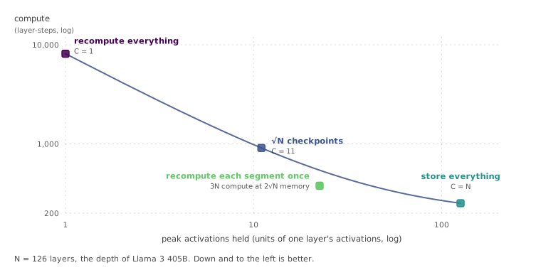
Activation checkpointing is genuinely a cost, not a free lunch — it makes every step slower, and the honest reason to turn it on is that the alternative is not training the model at all. It is the last of the memory techniques, and once it is enabled there are no more knobs of that kind. The remaining question is how to set the many knobs that now exist.

12.9 The metric that settles the arguments

Global batch size, local batch size, sharding-group size, replication factor, checkpoint interval, and shortly three more axes of parallelism: the configuration space is large, the interactions are not intuitive, and no amount of reasoning from first principles resolves it. What resolves it is a single measured number.

Build up to it in two steps. The first is hardware FLOPs utilisation, which asks what fraction of a device’s theoretical peak an operation actually achieves. An H100 is rated at 989.4 TFLOP/s of 16-bit matrix multiply on its tensor cores; a plain PyTorch loop multiplying dense square matrices reaches roughly 80% of that once the matrices are around $8192 \times 8192$, and considerably less when they are small. HFU is a property of the kernel and the shapes, and it is measured with a few lines of code.

HFU is also not the number that matters, because a training loop does a great deal that is not the matrix multiply: loading data, augmenting it, normalising, applying nonlinearities, communicating gradients, and — after Section 12.8 — recomputing activations it chose to throw away. Model FLOPs utilisation asks the sharper question: what fraction of the device’s theoretical peak is going into useful model computation?

It is computed as a ratio of times rather than of operations, which is what makes it robust. Count the matrix-multiply FLOPs in one forward and backward pass of your architecture on your batch, approximating the backward as twice the forward and ignoring nonlinearities, normalisation and elementwise operations, since those run on the FP32 cores and are not what the peak figure describes. Divide by the device’s rated throughput to get $t_\text{theoretical}$, the time the step would take on a perfect machine. Then measure $t_\text{actual}$, the wall-clock time of a complete iteration including data loading, forward, backward and the optimizer step. Then

$$\text{MFU} = \frac{t_\text{theoretical}}{t_\text{actual}} \tag{12.7}$$

Everything the training loop does other than the model’s own arithmetic lands in the denominator and nowhere else. Communication that failed to hide behind compute shows up here. So does a pipeline bubble, a straggler, a data loader that cannot keep up, and recomputation from activation checkpointing — which is the sharp consequence of Equation 12.7 worth pausing on. Recomputed FLOPs are real work the tensor cores perform, so they raise HFU; but they are not in the numerator of Equation 12.7, which counts one forward and one backward. Checkpointing therefore appears as a drop in MFU, correctly, because the extra work buys memory rather than progress.

Calibration: above 30% is good and above 40% is excellent. Well below 30% means something is badly wrong rather than slightly suboptimal, and is worth diagnosing before tuning anything.

Figure 12.7: BF16 model FLOPs utilisation for the three stages of Llama 3 405B pre-training, replotted from Table 4 of the Llama 3 paper. The drop from 43% to 41% comes from halving the per-group batch size to hold the global token count fixed while doubling the device count; the further drop to 38% is the cost of the long-context stage, which raises the sequence length sixteenfold and turns on context parallelism. Replotted for this project from published numbers.

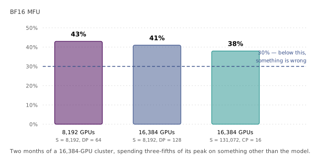
Llama 3 405B reached 43% on 8,192 GPUs, 41% on 16,384, and 38% in the final long-context stage. Those are state-of-the-art figures, and the shape of the decline is instructive: the 43% and the 41% differ only in that the second doubles the device count while holding the global tokens per batch constant, which halves the batch each data-parallel group sees and gives the collectives less arithmetic to hide behind.

One counterintuitive trend closes the section. Newer hardware sometimes achieves worse MFU than its predecessor. The A100 to H100 transition multiplied peak tensor-core throughput by about 3.2× — 312 to 989 TFLOP/s — while memory bandwidth roughly doubled. Compute is outrunning the ability to feed it, on the chip and between chips alike, so the fraction of a device’s peak that a real workload can reach has been drifting downward even as the absolute peak climbs. Every technique in the remainder of this chapter is aimed at that gap, and the gap is widening.

12.10 Tensor parallelism

Split the feature dimension, which means splitting a single weight matrix across devices. This is a different thing from FSDP, where a whole matrix has an owner and is temporarily copied elsewhere; here no device ever holds a complete $W$, and the matrix multiply itself is distributed.

A linear layer computes $XW = Y$ with $X$ of shape $N \times D$ and $W$ of shape $D \times D$. Cut $W$ into $P$ column blocks $W_1, \dots, W_P$, each $D \times D/P$, and give one to each device. Every device already has the full $X$, so device $i$ computes $XW_i = Y_i$, a column slice of the output, with no communication at all:

$$X \begin{bmatrix} W_1 & W_2 & \cdots & W_P \end{bmatrix} = \begin{bmatrix} Y_1 & Y_2 & \cdots & Y_P \end{bmatrix} \tag{12.8}$$

The forward pass of one layer is free. The trouble is the next layer, which appears to need all of $Y$, and gathering it would cost a full activation tensor per layer.

It does not need all of $Y$, provided the next layer is cut the other way. Let the second layer compute $YU = Z$ and split $U$ into $P$ row blocks $U_1, \dots, U_P$, each $D/P \times D$, with $U_i$ living on the same device as $W_i$. Block multiplication then gives

$$Z = YU = \sum_{i=1}^{P} Y_i U_i \tag{12.9}$$

and device $i$ already holds both factors of the $i$-th term. Each device computes a complete $N \times D$ partial sum from purely local data, and one all-reduce over the $P$ devices produces $Z$. Two layers, one collective.

Figure 12.8: Column-parallel followed by row-parallel. The first weight matrix is cut into column blocks, so each device produces a column slice of $Y$ and nothing needs to be exchanged. The second is cut into row blocks placed on the matching devices, so each computes one full-sized term of Equation 12.9 from data it already has, and a single all-reduce over the partial sums yields $Z$. Drawn for this project.

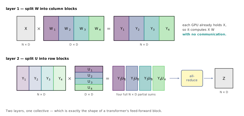
The pairing is not a coincidence looking for an application. A transformer’s feed-forward block is exactly two linear layers in sequence, so column-parallel then row-parallel drops onto it without modification, and tensor parallelism inside the MLP is standard practice in large transformers.

What tensor parallelism costs is bandwidth, and a lot of it: an all-reduce of a full activation tensor for every pair of layers, at every step, with the tensor cores stalled until it lands — there is no next layer to overlap it with. That places tensor parallelism firmly inside the fastest available domain. In practice the tensor-parallel degree is set to the number of GPUs in one server, so that every one of these collectives stays on NVLink and never touches the network.

12.11 Context parallelism

Split the sequence, so that several devices cooperate on a single long input. This is the axis that matters when the sequence length rather than the model size is what exhausts memory, which is the situation in long-context training and fine-tuning.

Most of a transformer takes to it easily. Normalisation, the feed-forward block and the residual connections all act on each token independently, so cutting the $S$ axis and handing each device a contiguous span of tokens changes nothing about their computation. The feed-forward block has weights, so its gradients need the same all-reduce that data parallelism required, but the forward pass is embarrassingly parallel.

Attention is not, and it is the entire difficulty. The queries, keys and values are per-token projections and split cleanly, but attention proper computes an interaction between every pair of positions, and a device holding tokens $1$ through $S/P$ needs keys and values from every other span to compute even one row of it.

Two answers exist. Ring attention keeps the sequence split and moves the data: the attention matrix is decomposed into blocks, and key–value blocks are passed around a ring of devices so that each device eventually sees every block it needs, with the transfers overlapped against the block computations. It is the more general solution and the more intricate one.

Ulysses attention is conceptually simpler and exploits a structure the architecture already has. Multi-head attention computes $H$ independent attention operations, so instead of splitting attention along the sequence, split it along the heads. An all-to-all before the attention block converts the sequence-sharded layout into a head-sharded one, each device computes a few complete heads over the full sequence, and a second all-to-all converts back. Everything outside attention stays split by sequence; only the attention operator changes its notion of what a device owns.

Llama 3 shows the regime where this becomes necessary. The first pre-training stage ran at a sequence length of 8,192 with no context parallelism at all. The final stage raised the sequence length to 131,072 and used 16-way context parallelism, putting sixteen GPUs on a single sequence — with 8,192 tokens each, which is exactly the span one GPU handled alone in stage one. The batch dimension has effectively gone below one example per device.

12.12 Pipeline parallelism

Split by depth: give the first quarter of the layers to GPU 1, the second quarter to GPU 2, and so on, passing activations across device boundaries in the forward pass and gradients back in the reverse. It is the most obvious partition of a deep network and, done naively, the worst.

The problem is the sequential dependency. GPU 2 cannot start until GPU 1’s output arrives; GPU 3 waits on GPU 2. The forward pass sweeps down the devices one at a time, GPU $P$ turns around and does its backward, and the gradients sweep back up, again one device at a time. At every instant exactly one device is working. With $P$ stages the utilisation ceiling is $1/P$, so eight-way pipeline parallelism caps MFU at 12.5% — worse than any bottleneck the previous sections were trying to fix. The idle regions have a name: the bubble.

The bubble exists because there is only one batch in flight, and the fix is to put several in flight. Split the batch into $m$ microbatches and stream them through the pipeline: GPU 1 runs forward on microbatch 1 and hands it to GPU 2, then immediately runs forward on microbatch 2 while GPU 2 works on microbatch 1, and so on. This is GPipe, and after a fill period of $P-1$ slots the pipeline is saturated.

Counting the schedule gives the utilisation directly. The forward sweep occupies $m + P - 1$ time slots and the backward sweep the same, for $2(m + P - 1)$ slots on $P$ devices, while the useful work is $2mP$ device-slots. So

$$\text{utilisation} = \frac{2mP}{2P(m + P - 1)} = \frac{m}{m + P - 1}, \qquad \text{bubble fraction} = \frac{P - 1}{m + P - 1} \tag{12.10}$$

With $m = 1$ this recovers the $1/P$ ceiling. With $P = 4$ and $m = 4$ it gives $4/7 \approx 57.1\%$, and the ratio keeps improving as $m$ grows.

Figure 12.9: A four-stage pipeline with four microbatches. Each colour is a microbatch; the shaded cells are the bubble. The fill and drain regions are what Equation 12.10 counts, and they shrink relative to the useful work as more microbatches are put in flight — which is why the only way to make pipeline parallelism efficient is to have many more microbatches than stages. Computed for this project.

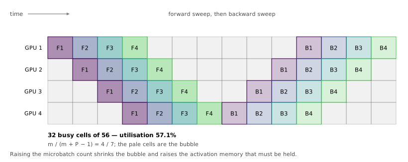
So take $m$ large and the bubble vanishes. Except that each in-flight microbatch holds its own activations until its backward pass completes, so raising $m$ raises activation memory in proportion — and the response to that is activation checkpointing, which costs compute, which costs MFU. More pipeline stages, fewer microbatches, more aggressive recomputation, more data parallelism layered on top: the knobs are coupled and there is no closed form for the optimum. This is what Section 12.9 is for. Tune whichever knob is available and keep the setting that maximises MFU.

12.13 Four dimensions at once

Which of the five strategies is best is the wrong question. The answer in practice is all of them, applied simultaneously along different axes, with the degree of each chosen to fit the cluster.

Arrange the GPUs conceptually in a grid with one dimension per parallelism strategy. A device’s coordinates give its rank along each axis: which shard of the feature dimension it holds, which span of the sequence, which block of layers, and which slice of the batch. HSDP in Section 12.7 was already a two-dimensional instance of this. Current practice runs four.

Llama 3 405B’s largest configuration is the concrete case. On 16,384 GPUs it used eight-way tensor parallelism, sixteen-way context parallelism, sixteen-way pipeline parallelism and eight-way data parallelism, and $8 \times 16 \times 16 \times 8 = 16{,}384$ accounts for every device exactly once.

The assignment of degrees to axes is where the topology of Section 12.3 is finally cashed in. Tensor parallelism is the most communication-hungry — an unhidden all-reduce of an activation tensor every two layers — and its degree is eight, which is precisely the number of GPUs in one server sharing an NVLink domain. Pipeline parallelism sends only a boundary activation tensor between adjacent stages and tolerates slower links, so it can span racks. Data parallelism communicates once per step and can span pods. The physical hierarchy that Figure 12.1 draws and the logical hierarchy of the parallelism grid are the same hierarchy, and the job of the configuration is to make them line up.

That, finally, is the discipline. There is no single trick and no schedule that is right in general. There is a machine with a known bandwidth hierarchy, a computation with four separable axes, one memory-for-compute trade, and one number that tells you whether the arrangement you chose is working.

12.14 Closing

A GPU is a parallel processor whose speed comes from a narrow specialisation — units that do nothing but small matrix multiply-accumulate at reduced precision — and whose performance is governed by a memory hierarchy in which everything larger is further and slower. A cluster is the same object at a larger scale, extending that hierarchy four levels past the edge of the chip, and it is best understood as one computer rather than as many.

Training a large model on it means splitting the computation along the four axes a transformer offers. The batch splits into data parallelism, and sharding the model state across the group turns that into FSDP, which trades three times the communication for an $M$-fold reduction in memory; restricting the sharding to the fast domain and replicating above it gives HSDP. The sequence splits into context parallelism, where everything but attention is trivial and attention needs ring or Ulysses. The feature dimension splits into tensor parallelism, where a column-parallel layer feeding a row-parallel layer needs one collective per pair and therefore belongs inside a server. The depth splits into pipeline parallelism, which is worthless without microbatches and good with them. Activation checkpointing sits underneath all of it, buying memory with recomputation at the $\sqrt{N}$ point where the two costs balance.

None of these choices has a principled optimum, and all of them are settled the same way — by measuring model FLOPs utilisation and keeping what raises it. The frontier sits between 38% and 43%, and it is not obviously going up, because compute is growing faster than the bandwidth that has to feed it.