13  Self-Supervised Learning

Lecture 12

Based on Lecture 12 of CS231n, Stanford University, Spring 2025.

13.1 What a representation costs

There is a result from earlier in the course that is easy to pass over and worth returning to. Take a network trained to classify ImageNet, cut it open at the last hidden layer, and read off the 4096-dimensional vector it produces for an image. Look for that image’s nearest neighbours in that vector space under an ordinary $L^2$ distance, and what comes back are pictures of the same kind of thing — the same animal in a different pose, against a different background, at a different scale. Do the same search in pixel space and what comes back are pictures with the same average colour.

The network was never asked to produce that. It was asked to name the object, and the vector is an artefact of the layer before the naming happens. Yet it is far more useful than the name: a linear classifier trained on those vectors will pick out categories the network was never shown, which is the whole content of the transfer learning discussed in Section 7.12. The representation is the valuable object, and the classifier on top of it is a thin thing that can be replaced.

Which raises the question of what the representation cost. It cost 1.2 million images, each of which a human being looked at and assigned to one of a thousand categories. That is the bill, and it grows steeply with how much detail the task demands. The COCO annotation effort is documented precisely enough to make the shape of the growth visible: deciding which of eighty categories appear in an image consumed about 20,000 aggregate worker hours across 328,000 images; marking where each instance sits added another 10,000; and drawing the actual outlines — 2.5 million of them, at over 22 worker hours per thousand — added roughly 55,000 more. The whole dataset took more than 70,000 hours of human attention, which is about forty years of one person working full time, and the segmentation stage alone is three quarters of it.

Figure 13.1: Aggregate human annotation effort per image, from published dataset papers. The first three bars are the three stages of the COCO pipeline and the last two are the two annotation qualities of Cityscapes; both papers report their own figures, and the axis is logarithmic because otherwise only the last bar is visible. The span from “which categories are present” to “every pixel has a class” is a factor of about twenty-five, and it is the reason dense prediction datasets are small.

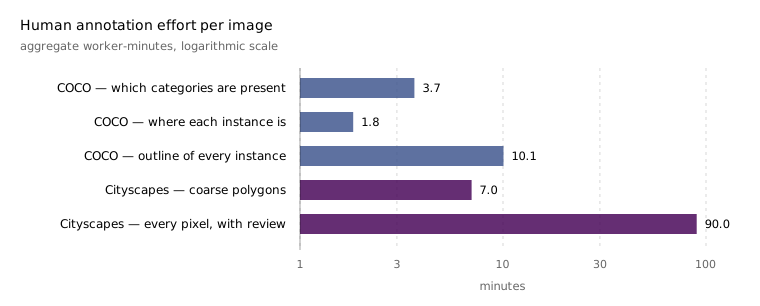
Push the density further and it gets worse rather than better. Cityscapes, which labels every pixel of a street scene with one of thirty classes, reports that annotation and quality control together required more than one and a half hours for a single image. The dataset’s coarse tier — polygons drawn quickly, deliberately not following boundaries — was capped at under seven minutes per image, and the fact that the authors built a second, worse tier at all is an admission that the good one does not scale.

Meanwhile there are, on the internet, some very large number of images that nobody has labelled and nobody is going to. The asymmetry is total: labelled data is a scarce, expensive, slowly-growing resource, and unlabelled data is effectively free and effectively unbounded. If the representation is the thing worth having, and the label is only the pretext under which it was obtained, then the question is whether some other pretext would do — one whose answers the data already contains.

13.2 An invented task, and a real one

The answer that organises this chapter is to invent a task. Take unlabelled images, corrupt or transform them in a way whose parameter you chose and therefore know, and train a network to recover that parameter. The supervision is genuine — there is a loss, a target, and a gradient, and the training is supervised learning in every mechanical respect — but no human produced the target. It was manufactured by the same code that produced the input. This is the pretext task, and the task you actually care about, trained afterwards on whatever small labelled dataset you have, is the downstream task.

The structure has two stages and one moving part between them. In the first stage a network is split into an encoder, which maps the image to a representation, and a head — a decoder, a classifier, a regressor, whatever the pretext task requires — which maps that representation to the manufactured target. Both are trained together on the unlabelled corpus. In the second stage the head is thrown away. The encoder is kept, a new and usually very shallow head is attached, and that head is trained on the labelled downstream data.

Figure 13.2: The two stages. Everything above the dashed line is trained on unlabelled data against a target the pipeline generated for itself; everything below is trained on a small labelled dataset. The encoder is the only thing that crosses. The pretext head exists solely to create a gradient and is discarded the moment it has done so, which is why its architecture matters much less than the loss it imposes on the encoder.

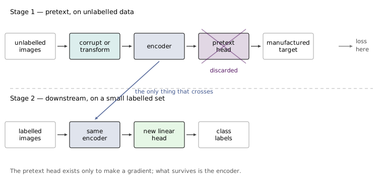
Discarding the head is not a detail. It is what makes the choice of pretext task a design problem rather than an application: nothing about solving the pretext task is wanted for its own sake, and the entire value of the exercise is in what solving it forces the encoder to encode. A pretext task can be perfectly solvable and completely useless, if there is a cheap surface statistic that solves it. Much of the history in Section 13.3 is the history of discovering such shortcuts and closing them.

That criterion also explains why the two requirements on a pretext task are stated together and are in tension. It must generate its own labels, which pushes towards simple mechanical corruptions; and solving it must require understanding the content of the image, which pushes towards corruptions no surface statistic can undo. The good pretext tasks sit where those two pressures meet.

Because the pretext task’s own accuracy is not the point, evaluating a self-supervised method takes some care, and three protocols recur throughout the rest of this chapter. Linear probing freezes the encoder entirely and fits a single linear layer on top using the full labelled training set. It asks a sharp question: are the classes already linearly separable in the representation, without any adaptation at all? Fine-tuning unfreezes everything and trains end to end from the pretext initialisation, which measures the representation’s value as a starting point rather than as a finished product. Semi-supervised evaluation fine-tunes on a deliberately small fraction of the labels — one percent, ten percent — which is the regime the whole enterprise is aimed at, since a method that only helps when you already have a million labels has not solved the problem it was built for.

These three do not agree with each other, and the places where they disagree are informative rather than noisy. A representation can be excellent under fine-tuning and mediocre under a linear probe, which says its information is present but not linearly accessible; Section 13.6 contains the sharpest instance of that gap. It is worth holding all three in mind, because papers tend to report the protocol that flatters them.

One last piece of context before the tasks themselves. Everything here is described for images, because this is a vision course, but self-supervised learning is not a vision technique that happens to work elsewhere. Predicting the next token in a corpus of text is a pretext task in exactly this sense — the label is the next word, which the data already contains — and it is the entire pre-training objective behind every large language model. The same pattern underlies modern speech models and much of what is now done in robotics, where the appeal is identical: a fleet collecting sensor data does not have to annotate it to learn from it. Vision arrived at the idea late and, for a while, awkwardly.

13.3 Tasks made from transformations

The first family of pretext tasks all have the same shape. Sample a transformation from some set, apply it to the image, and ask the network which one you applied. The transformation’s identity is the label, and it is free because you drew it yourself.

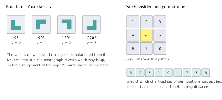
The cleanest instance is rotation. Rotate each image by one of $0°$, $90°$, $180°$ or $270°$ and train a four-way classifier on the result — this is RotNet, Gidaris et al., 2018. The restriction to multiples of a right angle is deliberate and does more work than it looks: those four rotations can be implemented as transposes and flips of the pixel array, so they introduce no interpolation artefacts and no border padding, and a network cannot solve the task by detecting resampling blur. It is a genuine four-way classification over image content.

The reason it can work at all is a hypothesis about what recognising an upright object requires. To know that a photograph of a dog has been turned on its side, you must know what an upright dog looks like — where the head sits relative to the legs, which way the ground is. There is no local statistic of a natural image that reveals its orientation; the information is in the arrangement of the object’s parts, and a network that solves the task has had to represent that arrangement.

Figure 13.3: The shared structure of the transformation tasks. On the left, one image and the four rotations it is turned into, each carrying the index of the rotation as its own label. On the right, the $3 \times 3$ patch grid: the relative-location task asks for one patch’s position among the eight around the centre, and the jigsaw task asks which of a fixed set of permutations was applied to all nine at once. In each case the label is drawn first and the image is manufactured from it, so the arrow between them runs the opposite way to ordinary supervision.

The evidence that it does is the transfer, and RotNet’s numbers are worth reading against the two baselines that bracket them. Pre-train an AlexNet on ImageNet with its labels, freeze it at conv4, and a classifier on those features reaches 59.7% top-1 on ImageNet; leave the same layers randomly initialised and frozen, and it reaches 27.1%. RotNet, which sees the same images and none of the labels, reaches 50.0%. The gap to the supervised ceiling is real, but the gap to random initialisation is four times larger, which is the finding. On PASCAL VOC 2007 detection the rotation-pretrained model reached 54.4% mAP, the best of any label-free method at the time.

A second finding from the same paper is more suggestive than the accuracies and easier to over-read. Visualising which regions each model’s activations respond to, the supervised classifier’s attention is narrow — it has found the parts that discriminate the thousand ImageNet categories and ignores everything else, which is exactly what its loss asked of it. The rotation model’s attention is spread over more of the object. That is not evidence of a better representation, since the model has no idea what the downstream task will be and has hedged accordingly; but a representation that hedges is the one you want when the downstream task is unknown, and this is the first appearance of a tension that runs through the chapter. A specific objective produces specific features. Self-supervision is trying to buy generality, and generality looks like this.

The second instance replaces rotation with spatial arrangement. Cut a $3 \times 3$ grid of patches from the image, hand the network the centre patch and one neighbour, and ask which of the eight surrounding positions the neighbour came from (Doersch et al., 2015). Again an eight-way classification, again free, again apparently requiring some idea of what the object is: to know that this patch of fur belongs above that patch of fur, you need to know it is a face.

Except that it does not require that, and the story of how it fails is the best illustration in this chapter of why pretext task design is hard. The first shortcut is obvious enough to be anticipated — patches that were adjacent in the original image have edges and textures that continue across the seam, so the network can match boundary patterns without looking at content. The fix is to leave gaps between the patches and jitter each patch’s position by a few pixels, and Doersch et al. did both. The second shortcut was not anticipated by anyone. Camera lenses focus different wavelengths at slightly different distances, so in many cameras the green channel is very slightly shrunk toward the image centre relative to red and blue. This chromatic aberration varies smoothly with distance from the optical axis, which means that measuring the local separation between green and magenta tells a network where on the lens a patch was taken from. Knowing each patch’s absolute position, the relative position is arithmetic. The network had learned to read the camera, not the scene.

The lesson generalises past this one bug. A pretext task defines a set of images the network must distinguish, and the network will find the cheapest feature that distinguishes them — not the feature you had in mind. Every advance in this family is, in part, the closing of a shortcut, and the eventual fix for chromatic aberration was to project colours away from the green–magenta axis or to drop two of the three channels outright and replace them with noise, both of which are ways of destroying information so the network cannot cheat with it.

Noroozi and Favaro’s jigsaw puzzles push the same idea to all nine patches at once: shuffle them and predict the permutation. All nine tiles have $9! = 362{,}880$ arrangements, which is too many classes to be usable and, worse, mostly indistinguishable — permutations differing in a single swap of two tiles pose an almost impossible discrimination. So the paper fixes a much smaller set of permutations in advance and predicts an index into it, which turns the problem back into a classification over a manageable number of classes. The set is not chosen at random: it is selected to maximise the average Hamming distance between its members, so that every permutation displaces most tiles and the network is never asked to split hairs. Chromatic aberration is handled here too, by jittering the colour channels. Solving the puzzle transfers about as well as relative patch prediction — 45.3% at conv4 against Doersch’s 45.6% — and the harder task did not buy much.

That flatness across the family is the honest summary. Rotation, relative location and jigsaw are three different inventions with three different shortcut problems, and they land within a few points of each other and well short of supervised pre-training. Each one buys features shaped by the peculiarities of its own task, and there is no principle telling you what to invent next.

13.4 Tasks made from reconstruction

The second family removes information from the image and asks the network to put it back. The label is the part you removed, so it is free in exactly the same sense; what differs is that the target is now a chunk of image rather than a class index, and that difference turns out to cause most of the trouble.

Cut a hole in the image and ask the network to fill it — context encoders, Pathak et al., 2016. The architecture is an encoder mapping the corrupted image to a representation and a decoder painting the missing region back, with the loss computed only where the hole was. Writing $M$ for the binary mask that is $1$ inside the hole and $0$ outside, and $F$ for the network,

$$L_{\text{rec}}(x) = \bigl\lVert M \odot \bigl(x - F((1 - M) \odot x)\bigr) \bigr\rVert_2^2 \tag{13.1}$$

where $\odot$ is elementwise multiplication. The network sees $(1-M) \odot x$, the image with its hole blacked out, and is scored only on $M \odot$ its output, the pixels it invented. To fill a hole convincingly the network has to know what object the surrounding context belongs to and what that object looks like where it cannot see, which is a strong demand and is why the task is interesting.

It is also where reconstruction losses first show their flaw. A hole in a photograph has many plausible fillings, and Equation 13.1 rewards the network for predicting their average. The average of many plausible fillings is a blur. Context encoders’ reconstructions are recognisably the right kind of content in the right place, and they are soft and smeared, and no amount of training fixes this because the smear is what the loss asked for. Pathak et al.’s remedy was to add an adversarial term — a second network trained to tell real images from filled-in ones, whose disapproval the first network must minimise — which converts “be close to the truth on average” into “be indistinguishable from something real”. The mechanics belong to Section 13.13’s successor lecture on generative models; what matters here is why it was needed.

Colourisation is the same idea applied to channels rather than regions, and it makes the ambiguity problem impossible to ignore. Convert the image to the Lab colour space, which factors a pixel into a lightness $L$ and two chrominance coordinates $a$ and $b$; hand the network $L$ and ask for $a$ and $b$. Every colour photograph in existence is a training pair, and the task genuinely needs semantics, since nothing in the grayscale intensities says a banana is yellow.

But an object’s colour is not determined by its shape. An apple may be red or green; a car may be any colour at all. Regressing $a$ and $b$ under a squared loss therefore drives the network to the mean of the plausible colours, and the mean of red and green is a muddy grey — which is precisely what the early colourisation networks produced. Zhang et al., 2016 diagnosed this and changed the output space rather than the architecture: quantise the $ab$ plane into a grid, keep the 313 cells that occur in natural images, and predict a distribution over those 313 classes with a cross-entropy loss. A distribution can be bimodal where a regression cannot, so the network is permitted to say “red or green, not grey”. A further reweighting compensates for the fact that most pixels in most photographs are near-neutral and would otherwise dominate the loss. The result is vivid colourisations, and the general lesson is worth extracting: when the target is genuinely ambiguous, the fix is usually to give the model a loss that can express the ambiguity, not to train it harder.

Once the task is stated as “given some channels, predict the others”, the restriction to $L \to ab$ looks arbitrary. Why not the reverse? The split-brain autoencoder does both at once: split the input tensor into two disjoint sets of channels $X_1$ and $X_2$, train one network $F_1$ to predict $X_2$ from $X_1$ and another network $F_2$ to predict $X_1$ from $X_2$, and use the concatenation of their representations as the feature.

Figure 13.4: The split-brain construction. A conventional autoencoder passes the whole input through a bottleneck and reconstructs it, which admits the degenerate solution of copying; splitting the channels makes each half a genuine prediction problem, because neither network can see what it is asked to produce. The two representations are concatenated, so the feature is defined on the whole tensor even though each encoder only ever saw part of it.

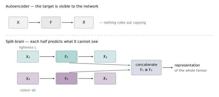
The split is what makes this more than a rebranded autoencoder. A plain autoencoder sees its own target and can, given enough capacity, learn to copy; every trick in the autoencoder literature is some way of preventing that. Withholding the channels being predicted removes the possibility structurally rather than by penalty. And because the construction refers only to “channels”, it applies wherever the input has more than one modality stacked: with an RGB-D sensor, predict depth from colour and colour from depth, and the concatenated feature has learned the relationship between geometry and appearance without anyone labelling either.

Where this family lands, measured on the same ImageNet probe as before, is around 40.7% at conv4 for colourisation against RotNet’s 50.0% and the fully supervised 59.7%. Reconstruction was competitive but not leading, and for several years the reasonable conclusion was that predicting pixels is a worse pretext task than predicting a discrete transformation parameter, because too much of the model’s capacity goes into reproducing texture that carries no semantic content. Section 13.6 is the story of that conclusion being overturned, and it was overturned by changing the architecture, not the objective.

13.5 Tracking, from nobody’s tracking labels

Everything so far uses the encoder afterwards and discards the mechanism that trained it. The most striking result in this lecture does the opposite: the mechanism is the useful thing, and it turns out to be a tracker that nobody asked for.

The setup is colourisation moved to video (Vondrick et al., 2018). One frame of a video is given in colour as a reference; the following frames arrive in grayscale, and the task is to colour them. Since objects keep their colour as they move, the answer for any target pixel is sitting somewhere in the reference frame — the problem is finding where.

The architectural decision that makes this work is a restriction. The network is not allowed to generate colour. It sees only grayscale, computes an embedding $f_i$ at every spatial location of both frames, and forms a soft correspondence between them by inner-product similarity,

$$A_{ij} = \frac{\exp\bigl(f_i^{\top} f_j\bigr)}{\sum_k \exp\bigl(f_k^{\top} f_j\bigr)} \tag{13.2}$$

where $i$ indexes reference locations, $j$ indexes target locations, and the softmax over $k$ makes each target location’s weights sum to one across the reference frame. The predicted colour is then nothing but a weighted average of reference colours,

$$y_j = \sum_i A_{ij}\, c_i \tag{13.3}$$

with $c_i$ the reference frame’s known colour at location $i$. This is precisely the attention of Section 9.4 — Equation 13.2 is a softmax over dot-product scores and Equation 13.3 is the weighted sum of values — with the reference frame supplying both keys and values and the target frame supplying queries. As in the single-image case the colour targets are quantised rather than regressed, here by $k$-means into sixteen clusters with a cross-entropy loss, for the same reason: an average of plausible colours is grey.

Figure 13.5: The pointer. Both frames enter as grayscale, so nothing in the network’s input carries colour; the only route from the reference colours to the prediction is the weight matrix $A$, and the loss can only be reduced by making $A$ point at the right place. What the network is forced to learn is therefore correspondence, and colour is merely the signal that reveals whether the correspondence was right.

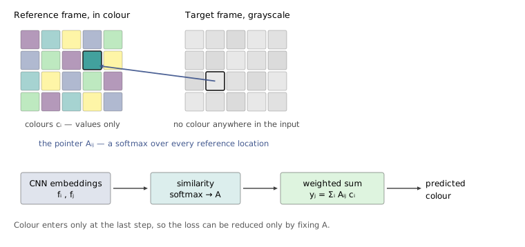
Because colour enters the prediction only through Equation 13.3, the loss can be reduced in exactly one way: by improving $A$. There is no capacity anywhere in the model for hallucinating a plausible colour from grayscale texture, which is what a colourisation network would ordinarily do. The gradient has a single path to travel, and it travels into the embedding that determines which reference pixel each target pixel points at. The network is trained on colour and learns correspondence, because correspondence is the only variable it has.

The payoff is that $A$ can carry anything. Take a video with one annotated first frame — a segmentation mask, or a set of pose keypoints — and propagate that annotation forward with the same Equation 13.3, substituting mask values or keypoint heatmaps for colours. The model has never seen a segmentation mask or a keypoint. It was trained on unlabelled video with a colour loss, and it tracks.

That is a genuinely different kind of result from the rest of this section. Rotation prediction gives you an encoder that you then have to train on something. Video colourisation gives you a working tracker as a side effect of a task that has nothing to do with tracking, which is what people mean when they say a capability emerges. The same phrase will recur in Section 13.12, for the same reason: a model trained with no notion of objects turns out to have found them anyway.

13.6 Masked autoencoders

Five years after context encoders concluded that pixel reconstruction makes a mediocre pretext task, masked autoencoders (He et al., 2021) reached the opposite conclusion with the same objective. Nothing changed about the loss — it is still mean squared error on the pixels that were removed. What changed is the architecture, and the change is worth understanding in detail, because it is the current default for pre-training vision models on raw data.

The image is cut into non-overlapping patches, exactly as in the ViT of Section 9.12. A large fraction of them — 75% in the default configuration — is sampled uniformly at random and discarded. What survives is fed to a Transformer encoder, and a decoder reconstructs the full image, with the loss computed only over the patches that were removed.

Two decisions inside that sentence carry the result.

The masking ratio is extreme. BERT masks 15% of tokens; MAE masks 75% of patches. The difference is not a hyperparameter tuned to a different value but a consequence of what the two media contain. A word is a nearly irreducible unit of meaning, and a missing word must be inferred from syntax and context. A $16 \times 16$ patch of a photograph is heavily redundant with its neighbours, and if only 15% are missing the task collapses into interpolation — extend the texture, continue the edge, done, with no understanding of the scene involved. Removing three quarters of the image destroys enough that local extrapolation cannot work and the network has to hold some model of what the object is. The difficulty is the point, and this is a general property of masking objectives: their value comes from being just solvable.

The encoder never sees a mask token. This is the structural asymmetry, and it is not obvious. The natural implementation would replace each removed patch with a learned placeholder and run the encoder over the full-length sequence. MAE does not. Removed patches are simply absent from the encoder’s input, so the encoder processes a quarter-length sequence of real image patches. Only the decoder assembles a full-length sequence, interleaving the encoded visible patches with copies of a single shared, learned mask token and adding positional embeddings so each one knows where it belongs. The decoder is deliberately small — the default has under a tenth of the encoder’s computation per token — and it is thrown away after pre-training, so its design is unconstrained by anything the downstream task needs.

Figure 13.6: The asymmetry. The encoder’s input sequence has length $vN$, where $v$ is the visible fraction, and the encoder is drawn tall because it is the heavy network; the decoder sees the full length $N$ and is drawn short because it costs under a tenth as much per token. Both the compute argument and the accuracy argument follow from where the sequence is short and where the network is heavy.

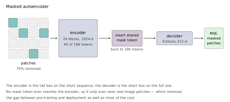
Both consequences of the asymmetry are large. The first is arithmetic. A Transformer block on $n$ tokens of width $d$ costs about $24nd^2$ in its projections and feed-forward and $4n^2d$ in the attention matmuls, so shortening the sequence by a factor of four makes the projections four times cheaper and the attention sixteen times cheaper. Evaluating that model for the paper’s actual configuration — a 24-block, 1024-wide ViT-L encoder, an 8-block, 512-wide decoder, 196 patches, 75% masked — gives a 3.3× reduction in total pre-training FLOPs against the same model with mask tokens in the encoder, which is exactly the figure the paper reports. The realised wall-clock speedup was 2.8×, and rose to 4.1× for a larger encoder with a one-block decoder.

Figure 13.7: Pre-training cost against masking ratio, evaluated from the per-block Transformer cost model in the figure’s generator for MAE’s ViT-L configuration. The encoder curve does bend — attention is quadratic in sequence length while everything else is linear — but only slightly, because at 196 tokens attention is just 3% of the encoder’s cost; the saving is overwhelmingly the linear term. The decoder cost is flat, since it always processes all 196 positions, which is why it has to be small. The two linear-probing accuracies the paper states in text are noted below the axis.

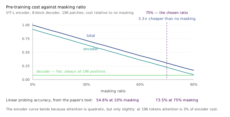
The second consequence is accuracy, and it is the less obvious of the two. Putting mask tokens into the encoder costs 14 points of linear-probing accuracy. The reason is a distribution mismatch: an encoder trained on inputs that are three-quarters placeholder is then deployed on uncorrupted images it has never seen, and the gap degrades it. Excluding mask tokens constrains the encoder to only ever look at real patches, so pre-training and deployment agree. Cheaper and better is an unusual combination, and it is what made the design stick.

The results justify the attention the method gets. A ViT-H pre-trained this way and fine-tuned on ImageNet-1K reaches 87.8% top-1, the best result at the time for any method using only ImageNet-1K data, and it beat the contrastive methods of Section 13.9 and Section 13.12 that had held the lead. For scale, a ViT-L trained from scratch on the same data reaches 82.5%; every masking ratio in the paper’s sweep beats that.

The ablations are where the divergence between evaluation protocols becomes impossible to ignore, and it is worth dwelling on. Under linear probing, accuracy climbs steadily with the masking ratio from 54.6% at the low end to 73.5% at 75% — a spread of nearly twenty points. Under fine-tuning, everything from 40% to 80% works about equally well and the total spread is under two points. Decoder depth behaves the same way: a deep decoder helps linear probing substantially and barely moves fine-tuning.

The explanation is that the two protocols measure different things, and the paper’s reading of it is convincing. The last layers of an autoencoder specialise in reconstruction, which is a pixel task rather than a recognition task. A deeper decoder absorbs more of that specialisation and leaves the encoder’s output more abstract — which is precisely what a linear probe needs, since a linear probe cannot undo a representation tilted toward pixels. Fine-tuning can undo it, so fine-tuning does not care. The practical warning is that linear probing is not a neutral measure of representation quality; it is a measure of linearly accessible quality, and a method optimised against it can be optimised in the wrong direction.

13.7 What all the pretext tasks were approximating

Step back from the individual methods and the shared weakness is easy to state. Every task in Section 13.3 and Section 13.4 had to be invented. Somebody noticed that rotation is recoverable, or that colour is separable, or that patches have positions, and each invention required its own analysis of what shortcut might defeat it. There is no procedure for generating the next one, and the features you get are shaped by the accidents of whichever task you happened to think of.

There is also a common thread running underneath all of them that none of them states directly. A rotated image is the same object as the unrotated one. A jigsaw permutation of an image is the same object. A grayscale image is the same object as its colour version, and a masked image is the same object as the whole. Every one of these tasks is an elaborate way of asserting that a particular transformation preserves identity — and then a specific pretext head is bolted on to force the network to notice.

So assert it directly. Take an image, produce two views of it by transformations that preserve what it depicts, and require the encoder to map them near each other. Take a different image, and require the encoder to map it far away. There is no head to design, no shortcut particular to one transformation, and no invention required beyond the choice of which transformations count as identity-preserving — which is a much smaller and more transferable design decision than inventing a task. That is contrastive representation learning, and it dominated the field from roughly 2019 onward.

13.8 The contrastive objective

Write $x$ for a reference image, $x^+$ for a view of the same image, and $x^-_1, \dots, x^-_{N-1}$ for views of different images. Let $f$ be the encoder and $s$ a scoring function on pairs of representations — in practice cosine similarity, scaled. What is wanted is

$$s\bigl(f(x), f(x^+)\bigr) \;\gg\; s\bigl(f(x), f(x^-)\bigr) \tag{13.4}$$

for every negative. Turning that wish into a differentiable loss is done by the standard device: exponentiate the scores, normalise, and take the negative log probability of the positive,

$$L = -\log \frac{\exp\bigl(s(f(x), f(x^+))\bigr)}{\exp\bigl(s(f(x), f(x^+))\bigr) + \sum_{j=1}^{N-1} \exp\bigl(s(f(x), f(x^-_j))\bigr)} \tag{13.5}$$

which is exactly the cross-entropy of an $N$-way softmax classifier whose correct answer is always index zero. The network’s job, restated, is to pick the positive out of a lineup of $N$ candidates. Nothing here is new machinery — Equation 13.5 is the softmax loss of Section 3.6 with the classes redefined at every step — and that is the appeal, since all the optimisation behaviour is already understood.

Figure 13.8: The lineup. One anchor, one positive that is another view of the same image, and $N-1$ negatives drawn from other images. The gradient of Equation 13.5 pulls the positive toward the anchor and pushes every negative away, with each negative’s push weighted by how much probability mass it currently steals — so a negative that is already far away contributes almost nothing, and the hard ones dominate.

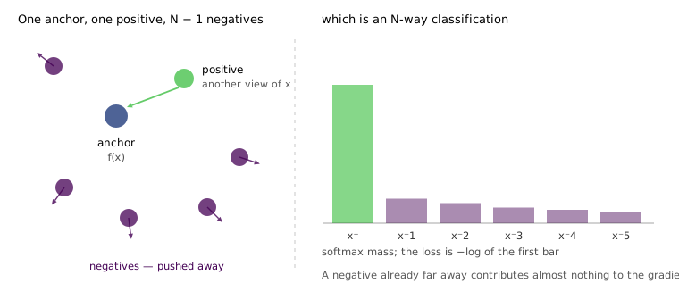
Equation 13.5 is the InfoNCE loss, introduced with the contrastive predictive coding paper of van den Oord et al., 2018, and its name records a claim about what it does. Mutual information $I(x; x^+)$ measures how much knowing one variable tells you about the other. The paper shows that

$$I(x; x^+) \;\ge\; \log N - L_N \tag{13.6}$$

where $L_N$ is the InfoNCE loss at $N$ samples. Since the loss appears negated, minimising it raises a lower bound on the mutual information between the two views — which is a satisfying story, because “keep whatever the two views share and discard whatever they do not” is a reasonable description of what a good representation should do.

Equation 13.6 is also where the argument for enormous batches comes from, and it is worth stating more carefully than it usually is. $L_N$ is a cross-entropy and so is never negative, which means the right-hand side of Equation 13.6 never exceeds $\log N$. The bound cannot certify more than $\log N$ nats of mutual information no matter how good the encoder becomes: with $N = 256$ that ceiling is about 5.5 nats, and it is a property of the objective rather than of the model. Increasing $N$ is the only way to raise it. That is a sharper claim than “more negatives tighten the bound”, and it explains why the methods in the next two sections are so preoccupied with where to get more negatives from — the whole engineering effort in Section 13.9 and Section 13.10 is aimed at this one term.

One caveat belongs here, because the mutual-information framing is more often repeated than examined. Later analyses (Tschannen et al., 2020) found that tighter mutual-information estimators do not produce better representations, and that the success of these methods depends heavily on the encoder architecture and on which transformations generate the views — neither of which appears anywhere in Equation 13.6. The bound is a genuine theorem and a good motivation; it is not an explanation of why contrastive learning works. Treat the $\log N$ ceiling as the reliable part.

13.9 SimCLR

SimCLR (Chen et al., 2020) is Equation 13.5 with the three remaining blanks filled in as simply as possible, and its contribution is largely the demonstration that filling them in carefully is enough.

Positives come from augmentation. Each image in the batch is passed through two independently sampled augmentations — random resized crop, colour distortion, Gaussian blur — producing two views. The two views of one image are a positive pair; every other view in the batch is a negative. A batch of $N$ images therefore yields $2N$ encoded views, each of which takes a turn as the anchor, giving $2N - 2$ negatives per anchor.

Which augmentations are used turns out to matter enormously, and the paper’s ablation of this is its most useful practical finding. Random cropping alone is weak; colour distortion alone is weak; the composition of the two is what works. The reason is a shortcut of the sort Section 13.3 was full of. Two crops of the same photograph share a colour histogram, and a network can match them on that alone without looking at content at all. Distorting the colours independently in each view destroys the shortcut and forces the match to be made on structure.

The score is cosine similarity between $\ell_2$-normalised embeddings, divided by a temperature $\tau$, which gives the NT-Xent loss — normalised temperature-scaled cross entropy. The normalisation removes vector magnitude from the comparison and the temperature controls how sharply the softmax in Equation 13.5 distinguishes hard negatives from easy ones; both matter, and the paper ablates both.

The third blank is where the loss is applied, and here SimCLR does something that looks redundant and is not. The encoder produces a representation $h$; a small MLP projection head $g$ maps $h$ to a second vector $z$; and the contrastive loss is computed on $z$. Then the projection head is discarded and $h$ is what gets used downstream. Training on one layer and deploying a different one is strange until you ask what the loss does to whatever it acts on. Equation 13.5 demands invariance to the augmentations, so it will happily destroy any information the augmentations changed — colour, orientation, scale. That is exactly right for the objective and often wrong for the downstream task, which might well need to know what colour the object is. Interposing the head gives the loss a layer to flatten while leaving $h$ upstream of the damage, and the measured gap between using $h$ and using $z$ is substantial.

The results were the ones that made the field pay attention. Linear probing on SimCLR features from a ResNet-50 (4×) reaches 76.5% top-1 on ImageNet, which matches a supervised ResNet-50 trained with all the labels; the same method on an ordinary ResNet-50 gets 69.3%, and the gap is the price of generality — a representation that has to serve unknown tasks needs more capacity than one aimed at a thousand known classes. Fine-tuned on 1% of ImageNet’s labels it reaches 85.8% top-5, beating AlexNet trained on all of them.

The cost is where the $\log N$ ceiling of Equation 13.6 shows up as an engineering bill. SimCLR’s negatives all come from the current batch, so raising $N$ means raising the batch size, and the paper’s best configurations use batches of 4096 and 8192 — the latter giving 16,382 negatives per positive. A batch that size does not fit on one accelerator, needs distributed training and the LARS optimiser to remain stable, and puts the method out of reach of anyone without a TPU pod. The negatives and the batch are welded together, and that is the flaw the next method attacks.

13.10 MoCo

Momentum contrast (He et al., 2020) observes that the coupling is an implementation accident rather than a requirement. A negative only needs to be an encoded view of some other image; nothing says it has to have been encoded during this step. So keep a queue.

Figure 13.9: Where the negatives come from. SimCLR draws them from the current batch, so the negative count and the batch size are the same number and both are bounded by memory. MoCo maintains a FIFO queue of encoded keys that is orders of magnitude larger than the batch, enqueuing the current batch and evicting the oldest. Gradients flow only along the query path — the dashed path carries none — which is what makes the queue affordable and also what creates the problem the momentum update solves.

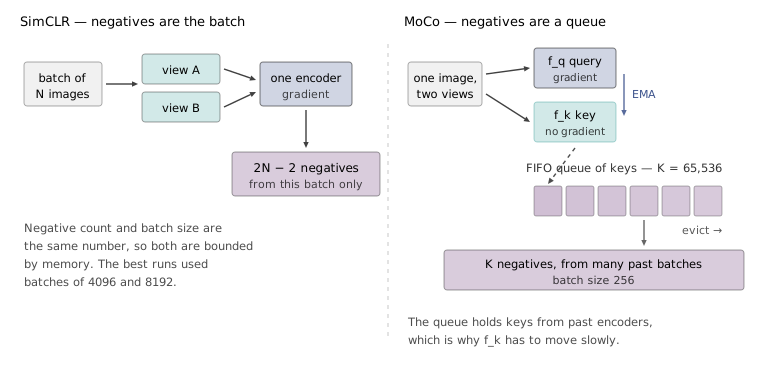
Concretely: one view of each image becomes a query, encoded by $f_q$; the other becomes a key, encoded by $f_k$. Keys are pushed into a FIFO queue as each batch is processed and the oldest are evicted, so the queue holds keys from many recent batches — MoCo uses 65,536 of them with a batch size of 256. The InfoNCE loss compares the query against its own key and against everything in the queue.

Backpropagation through the queue is impossible: those keys were produced several steps ago, their activations are long gone, and storing them would defeat the memory saving entirely. So the key path carries no gradient at all, and only $f_q$ is updated by the optimiser. Which leaves the question of where $f_k$ comes from.

Making $f_k$ a copy of $f_q$ — recopied after every optimiser step — does not work, and the reason is the crux of the method. The queue holds keys produced by whatever $f_k$ was at the time each key was enqueued. If $f_k$ changes quickly, keys near the front and keys near the back of the queue were produced by encoders that disagree, and comparing a single query against all of them is comparing against an incoherent dictionary. Similarities computed against inconsistent keys carry no reliable signal.

The fix is to make $f_k$ change slowly, by an exponential moving average of the query encoder:

$$\theta_k \leftarrow m\,\theta_k + (1 - m)\,\theta_q \tag{13.7}$$

with $m$ close to one. The ablation makes the argument better than any explanation does. At $m = 0$ — the naive copy — training oscillates and fails to converge. At $m = 0.9$ the model reaches 55.2%; at $m = 0.99$, 57.8%; at $m = 0.999$, 59.0%. A hyperparameter whose useful range is between three and four nines is not being tuned, it is being used to enforce a constraint, and the constraint is that the dictionary must be self-consistent.

MoCo v2 is the unsurprising and effective conclusion: take SimCLR’s MLP projection head and stronger augmentation, keep MoCo’s queue and momentum encoder, and the combination beats SimCLR while training with a batch of 256 instead of 8192. That is the practical summary of this pair of papers. The projection head and the augmentation policy were the ideas; the queue was the engineering that made them affordable on ordinary hardware.

13.11 Contrasting sequences instead of instances

SimCLR and MoCo are instance contrastive learning: the unit of identity is one image, and positives are views of it. Contrastive predictive coding — the paper that introduced Equation 13.5 in the first place — contrasts along a different axis. The unit is a position in a sequence, and the positive is what actually comes next.

The construction has three parts. An encoder maps each element of the sequence to a latent, $z_t = g_{\text{enc}}(x_t)$. An autoregressive model, a GRU in the original paper, summarises everything up to the present into a context vector $c_t = g_{\text{ar}}(z_{\leq t})$. And then, for each prediction offset $k$, a bilinear score

$$s_k(x_{t+k}, c_t) = z_{t+k}^{\top} W_k\, c_t \tag{13.8}$$

is fed to Equation 13.5, with the true future latent $z_{t+k}$ as the positive and latents drawn from elsewhere in the data as negatives. A separate $W_k$ per offset lets the model predict differently at different horizons, which it must, since one step ahead and twelve steps ahead are different problems.

The design decision worth extracting is that the prediction happens in latent space, not in the data. A model that predicted the actual future waveform or the actual future pixels would have to spend most of its capacity on the high-frequency detail that dominates those signals and carries almost none of the structure — the same complaint Section 13.4 raised about reconstruction losses. Scoring a latent against a context sidesteps this: the model never has to represent $p(x_{t+k})$, only to tell the real continuation from an impostor, and it can discard whatever detail does not help with that discrimination.

The formulation is indifferent to what the sequence contains. On audio it is applied directly to a waveform, and a linear classifier on the resulting representations recovers phonemes and speaker identity. On images the sequence has to be manufactured: cut the image into a grid of patches, read the rows top to bottom as if they were time, and use the upper rows as context for predicting the lower ones. That works, and it is worth being clear that it works less well than the instance-level methods — an image has no intrinsic ordering, and imposing one throws away the two-dimensional structure that convolutions and attention exploit. CPC’s importance to vision is mostly that its loss function outlived its architecture.

13.12 DINO, and doing without negatives

Everything since Section 13.8 has been organised around negatives, and negatives are a nuisance: they are what forces the batch to be enormous or the queue to exist, and they are semantically wrong in an obvious way, since two different images of dogs are treated as things that must be pushed apart. DINO (Caron et al., 2021) does without them.

The frame is knowledge distillation with nothing to distil from. Two networks with identical architecture, a student $g_{\theta_s}$ and a teacher $g_{\theta_t}$, each map an image to a $K$-dimensional distribution through a softmax. Two augmented views of the same image are produced; the student sees one, the teacher the other; and the student is trained to match the teacher’s output distribution under cross entropy. Gradients flow only through the student — the teacher carries a stop-gradient — and the teacher’s weights are an exponential moving average of the student’s, the same Equation 13.7 that MoCo used. The teacher is the student’s own recent past, which is why the method’s name expands to self-distillation with no labels.

Nothing in that description prevents the trivial solution. A student and teacher that both emit the same constant distribution for every image achieve zero loss and have learned nothing. Every method in this chapter has some device for ruling that out — contrastive learning uses negatives, which make a constant output maximally wrong — and DINO’s device is two operations on the teacher’s output that are individually harmful and jointly sufficient.

Figure 13.10: The two failure modes and the two corrections. Collapse can be to a single dominant dimension or to the uniform distribution, and the two fixes push in opposite directions: centring subtracts a running mean of teacher outputs, which stops any dimension from dominating but drives everything toward uniform; sharpening uses a low softmax temperature on the teacher, which drives outputs away from uniform but toward a single dimension. Neither alone is stable. Applied together they hold the output between the two collapses.

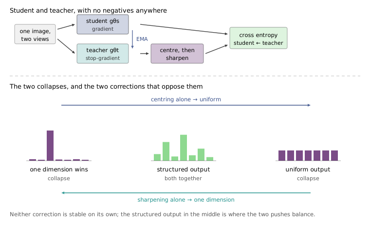
Centring maintains a running mean $c$ of teacher outputs across the batch, updated by its own moving average, and subtracts it before the softmax. This stops any single output dimension from dominating, but on its own it pushes the teacher’s distribution toward uniform — which is the other collapse. Sharpening uses a low temperature in the teacher’s softmax, concentrating the distribution, which pushes away from uniform but on its own encourages exactly the one-dimension domination that centring exists to prevent. The two corrections have opposite biases and neither is stable alone; run together, they balance, and no negatives are needed. It is a genuinely different mechanism from Equation 13.5, which is why DINO is often described as contrastive-adjacent rather than contrastive.

One more component matters for what emerges. DINO uses multi-crop: the teacher sees large global crops and the student sees several small local ones, and the student must predict the global view’s distribution from a local patch. That is a local-to-global objective, and it forces the representation of a small region to carry information about the whole object it belongs to.

The results include the best pure-feature numbers of the chapter. A $k$-nearest-neighbour classifier on frozen DINO features — no training of any kind on top, just look up the nearest neighbours and vote — reaches 78.3% top-1 on ImageNet, which is a much stronger claim than a linear probe, since a $k$-NN classifier has no parameters to fit and can only work if the representation’s geometry is already right. Linear evaluation with a ViT-Base reaches 80.1%.

And then the property the paper is named for. Visualising the attention of the ViT’s class token in a DINO-trained model shows it attending to object boundaries — the segmentation of the scene is present in the attention maps, sharply enough to be used, and it does not appear this clearly in a ViT trained with ImageNet labels or in a convnet. Nothing in the training objective mentions objects, segmentation, or spatial extent. This is the second time in this chapter that a capability nobody trained for turned up anyway, after Section 13.5, and the two cases share a shape: an objective that forces a model to relate one part of an image to another leaves behind a machine for finding those relations, and the machine is usable for things the objective knew nothing about.

DINOv2 scaled the recipe — much more data, curated rather than scraped, and a larger model — into features good enough to be used frozen across depth estimation, segmentation and retrieval without task-specific fine-tuning, which is close to the original promise of Section 13.1: train once on unlabelled images, use the representation everywhere.

13.13 Where this leaves things

Two families came out of this lecture and both are alive. Reconstruction, dismissed in 2016 and rehabilitated by Section 13.6’s architectural asymmetry, learns by predicting the parts of the input it was not shown. Joint-embedding methods — contrastive in Section 13.9 and Section 13.10, distillation-based in Section 13.12 — learn by requiring two views of one thing to agree, and never model pixels at all. They have different failure modes, different costs, and different downstream profiles: masked autoencoders fine-tune superbly and probe indifferently, joint-embedding methods produce representations that are linearly separable and even nearest-neighbour separable straight out of the box.

What has not survived is the part of the lecture that came first. Nobody now designs a rotation-prediction task, and the reason is worth keeping: hand-designed pretext tasks buy features shaped by the accidents of the task, and the two surviving families both replaced the invented task with a statement about what the data is — that an image is redundant enough to be reconstructed from a quarter of itself, or that two views of one scene depict one thing. Those are claims about images rather than puzzles about them, which is why they generalise.

The thread running through both is that supervision was never really the scarce resource; labels were. Everything here is supervised learning in the mechanical sense — a target, a loss, a gradient — and the whole contribution is arranging for the target to be something the data already knows. That is also what the next lecture is about from a different direction: a generative model, asked to produce samples from the distribution of natural images, is solving the hardest version of the same problem, and its representations come from the same place.