8  Recurrent Neural Networks

Lecture 7

Based on Lecture 7 of CS231n, Stanford University, Spring 2025.

8.1 Problems with a shape

Every network in the preceding chapters commits to a shape when it is built. A convolutional classifier accepts an image of fixed height and width and emits a vector of fixed length, one score per class, and both of those numbers are decided before a single weight is learned. That commitment is not a limitation anyone had to work around, because the problem was itself shaped that way: classification takes one image and returns one label.

A great many problems are not shaped that way, and they fail the commitment in different places. Captioning takes a single image — a fixed-size input, no trouble there — and must return a sentence, whose length is not known until the sentence is finished. Classifying an action in a video is the mirror image: the input is a run of frames of no fixed number, and the output is a single label. Translation varies at both ends and, worse, varies at the two ends independently, since a sentence and its translation need not have the same number of words. Labelling every frame of a video with what is happening in it varies at both ends too, but in lockstep, one output for each input.

Figure 8.1 draws the five patterns. It is tempting to read them as five architectures, and they are not; they are five ways of attaching inputs and losses to one machine. The machine has to consume input incrementally and produce output incrementally, and once it does, whether a particular input step carries a real vector or a placeholder, and whether a particular output step is scored or discarded, is a decision made per problem rather than per model. This chapter develops the machine on the rightmost pattern, where every step has both an input and a scored output, because that is where the mechanics are least cluttered. The others follow by changing what is attached where.

Figure 8.1: The five ways a problem can be shaped, and where each one breaks the fixed-size commitment. Indigo blocks below are inputs, teal blocks above are outputs, and the grey band between them is the network. Only the first is served by a feedforward network; the other four need a model that can consume and emit one step at a time. The rightmost two both vary at input and output, but the last aligns them one to one, which is why it is the easiest to reason about. Drawn for these notes.

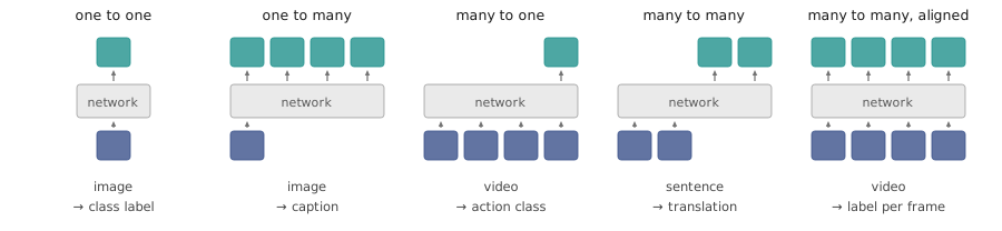
Note what the shapes do not distinguish. Nothing here says the input steps are moments in time. They are for video and for speech, but for a sentence the steps are positions in a string, and for a program they are tokens in a file; the ordering is real and the metric structure is not. “Time step” is the conventional name and this chapter uses it, but the only property the model actually relies on is that the steps come in an order and that order carries meaning.

8.2 A state that persists

If the network is to read a sequence one element at a time and its behaviour at step $t$ is to depend on what came before, then something must survive between steps. Call it the hidden state $h$, a vector the network carries forward and rewrites at each step. Then the whole model reduces to a single line:

$$h_t = f_W(h_{t-1},\, x_t) \tag{8.1}$$

where $x_t$ is the input at step $t$, $h_{t-1}$ is the state left over from the step before, and $f_W$ is a function with parameters $W$. This is the recurrence, and it is the entire idea. Everything else in this chapter is a choice of $f$, a choice of where to attach losses, or a consequence of the fact that Equation 8.1 is applied over and over.

The subscript on $f_W$ deserves attention, because there is only one of them. The same function with the same parameters runs at step 1, at step 40 and at step 4000. This is not a simplification adopted for convenience; it is what makes the model well defined at all. A network with a distinct $W_t$ per step would have a parameter count that grows with sequence length, would need to be rebuilt for every new length, and — decisively — could not apply anything it learned at step 5 to step 500, because the weights that fire at step 500 would never have been touched by a training sequence of length 40. Sharing the weights across time is the same argument that made a convolutional filter slide across an image in Section 6.11, moved from space to order: a pattern worth detecting is worth detecting wherever it occurs, so the detector should not be indexed by where it looks.

The state is not the output. It is an internal quantity, and turning it into whatever the task actually wants is a second function with its own parameters:

$$y_t = f_{W_{hy}}(h_t). \tag{8.2}$$

Two things are happening in Equation 8.2 and they are worth separating. The obvious one is dimensional: $h_t$ lives in whatever space the designer chose for it, typically a few hundred dimensions, and $y_t$ has to live in the space the task defines — one score per class, or one score per word in a vocabulary. The less obvious one is that the map is learned, so it is not merely a projection into the right shape but a transformation the network can tune. The division of labour is that $f_W$ decides what is worth remembering and $f_{W_{hy}}$ decides how to read it out, and those are different jobs.

Fixing the two functions to the simplest thing that could work gives the model that everyone means by vanilla RNN, and, after the psycholinguist who introduced this architecture in 1990 (Elman), the Elman network:

$$h_t = \tanh\!\left(W_{hh}\,h_{t-1} + W_{xh}\,x_t\right), \qquad y_t = W_{hy}\,h_t . \tag{8.3}$$

Three weight matrices, each doing one job. $W_{xh}$ maps an input vector into the hidden space; $W_{hh}$ maps the previous hidden state into the hidden space; the two results are added, and a nonlinearity is applied to the sum. $W_{hy}$ maps the result out. Bias terms are omitted here and are present in every implementation.

The choice of $\tanh$ rather than the ReLU that Section 7.4 settled on elsewhere is deliberate and specific to recurrence. In a feedforward network an activation is applied a fixed number of times, once per layer, and if ReLU lets values grow that growth is bounded by depth. Here the same nonlinearity is applied once per step, and the number of steps is a property of the data. A function whose output is bounded to $[-1, 1]$ keeps the state in a fixed range no matter how long the sequence runs, which an unbounded activation does not; that it is also zero-centred, and so can represent a quantity being pushed in either direction, is the second reason. Both of these will look different by the end of the chapter — bounding the state turns out to cost something on the backward pass — but the reasoning is sound as far as it goes.

8.3 A network built by hand

The equations above are short enough to hide how little is going on inside them. It is worth doing one recurrence completely, with numbers, and the clearest way is to abandon learning entirely and set the weights by hand for a task small enough to solve in one’s head.

The task: read a sequence of zeros and ones, and emit $1$ at any position where the current input and the previous input are both $1$, and $0$ everywhere else. This is the aligned many-to-many shape — one output per input — and it is the smallest problem that genuinely requires memory, since the correct output at step $t$ is not a function of $x_t$ alone.

Start by asking what the hidden state has to hold. The output at step $t$ depends on $x_t$ and on $x_{t-1}$, and the state is the only channel through which anything from the past can arrive, so the state must carry $x_{t-1}$. Since the output is computed from the state alone, it must carry $x_t$ as well. Two numbers, then; take three, laying out the state as

$$h_t = \begin{pmatrix} \text{current} \\ \text{previous} \\ 1 \end{pmatrix}, \qquad h_0 = \begin{pmatrix} 0 \\ 0 \\ 1 \end{pmatrix} . \tag{8.4}$$

The constant $1$ in the third slot is a bias smuggled into the state vector so that the readout can subtract a threshold without a separate bias term, and the initial state asserts that the sequence is preceded by zeros. Replace $\tanh$ with a ReLU, purely so every quantity below is an integer.

Now build the two matrices. The input contributes to the state through $W_{xh}$, which here maps a scalar to three dimensions and needs to place $x_t$ into the first slot and nothing anywhere else:

$$W_{xh} = \begin{pmatrix} 1 \\ 0 \\ 0 \end{pmatrix}, \qquad W_{xh}\,x_t = \begin{pmatrix} x_t \\ 0 \\ 0 \end{pmatrix}. \tag{8.5}$$

The old state contributes through $W_{hh}$, which has to do three separate things at once, one per row. The first row must be zero, because the new “current” slot comes entirely from the input and must not inherit anything. The second row must copy the old first slot into the new second slot — last step’s current becomes this step’s previous. The third row must preserve the constant. Writing that down:

$$W_{hh} = \begin{pmatrix} 0 & 0 & 0 \\ 1 & 0 & 0 \\ 0 & 0 & 1 \end{pmatrix}, \qquad W_{hh} \begin{pmatrix} c \\ p \\ 1 \end{pmatrix} = \begin{pmatrix} 0 \\ c \\ 1 \end{pmatrix}. \tag{8.6}$$

Adding the two contributions and applying the ReLU, which changes nothing because every entry is already non-negative, gives $h_t = (x_t,\; c_{t-1},\; 1)^\top$ — exactly the layout Equation 8.4 asked for, with the state shifted along by one position. The two matrices have divided the work cleanly: $W_{hh}$ carries information forward from the past, and $W_{xh}$ injects the present. That division is not an artefact of the toy problem. It is what those two matrices are always doing, in every RNN, however large.

The readout is a single row, since the output is one number:

$$W_{hy} = \begin{pmatrix} 1 & 1 & -1 \end{pmatrix}, \qquad y_t = \operatorname{ReLU}\!\left(W_{hy} h_t\right) = \max\!\left(c_t + p_t - 1,\; 0\right). \tag{8.7}$$

This is where the constant earns its slot: the $-1$ multiplies it, and the expression $c + p - 1$ is positive only when $c$ and $p$ are both $1$, in which case it equals $1$. Two ones give $1$; a one and a zero give $\max(0, 0) = 0$; two zeros give $\max(-1, 0) = 0$. The ReLU has been turned into a logical AND.

Run it on $0,1,0,1,1,1,0,1,1$ and the states go $(0,0,1)$, $(1,0,1)$, $(0,1,1)$, $(1,0,1)$, $(1,1,1)$, $(1,1,1)$, $(0,1,1)$, $(1,0,1)$, $(1,1,1)$, and the outputs $0,0,0,0,1,1,0,0,1$, which is the answer. The network is nine parameters and detects a pattern no fixed-size classifier over a single input could.

Two things about this example are honest and one is not, and it is worth being clear which is which. The mechanics are exactly those of a real RNN: the same matrices multiply the same way, and a hidden state of three hundred dimensions runs the identical computation. What is unreal is the provenance of the weights. Nobody finds $W_{hh}$ by staring at the problem; a real network is trained, and a hidden state large enough to be useful holds distributed quantities that correspond to no slot anyone named. Getting there requires computing gradients through a computation whose length is a property of the input, which is the subject of the next section.

8.4 Unrolling

The loop in Equation 8.1 is a loop only in the way it is written. Executed on a sequence of $T$ elements it produces a chain of $T$ applications of $f_W$, each consuming the state the last one produced, and that chain is an ordinary directed acyclic graph of the kind Section 5.8 handled. Drawing it that way is called unrolling, and it is what makes the model differentiable by machinery already in hand: there is no new rule for recurrent networks, only an old rule applied to a graph whose size depends on the input.

Figure 8.2: The recurrence as written and the recurrence as executed. On the left, the loop notation, with the arrow that feeds the state back into the block; on the right, the same computation unrolled over four steps. The single box $W$ at the bottom, with an edge into every application of $f_W$, is the whole difference between this graph and a four-layer feedforward network: the same parameters are consumed four times, so on the backward pass four gradient contributions arrive at the same node and are summed. Drawn for these notes.

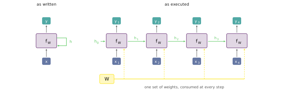
Figure 8.2 makes the one genuinely new thing visible. $W$ is a single node with an edge running into every step, so it is a variable used $T$ times, and the multivariable chain rule says that the gradient arriving at a node used several times is the sum of the contributions along each use:

$$\frac{\partial L}{\partial W} = \sum_{t=1}^{T} \left.\frac{\partial L}{\partial W}\right|_{\text{step } t}. \tag{8.8}$$

This is worth stating because it is the point at which people expect something exotic and get arithmetic instead. Backpropagation through a shared weight is the same operation as backpropagation through a residual connection or through any other fan-out in a graph: contributions add. One useful way to hold it is to pretend, while working backwards, that each step has its own private copy $W_1, \dots, W_T$, compute the $T$ gradients independently, and only at the end remember that all $T$ copies are the same array and add them together. Applied to a recurrent network this procedure has a name of its own, backpropagation through time, though it introduces no rule that Section 5.11 did not already contain.

Where the loss enters depends on which of the shapes from Section 8.1 is in play, and the four cases differ only in what is attached to the graph rather than in the graph itself. In the aligned many-to-many case every step produces an output, every output is scored, and the total is

$$L = \sum_{t=1}^{T} L_t , \tag{8.9}$$

with each $L_t$ typically a cross-entropy against the target at that position. Because the sum is over independent terms, the gradient of $L$ decomposes into one contribution per step before Equation 8.8 ever gets involved.

Many-to-one is the case with a single loss at the end, and it is the more instructive of the two. Only $h_T$ feeds the output, so the intermediate hidden states receive no gradient of their own; everything that reaches step 5 has travelled backwards from step $T$ along the chain of state transitions. The states are still on the path, and they still get gradients, but those gradients are entirely upstream in origin. It is worth noting that using $h_T$ alone is a choice, not a requirement: for video classification the frames near the beginning may carry as much evidence as the frames near the end, and pooling the hidden states across time before the readout is a common and often better alternative to reading only the last one.

One-to-many exposes a small gap in Equation 8.1. The recurrence needs an $x_t$ at every step because $W_{xh}x_t$ is a term in it, but a captioning model has exactly one real input, the image, and $T-1$ steps with nothing to consume. Two answers are in use. Feeding zeros is the honest admission that there is no input; feeding the model’s own previous output, $x_t = y_{t-1}$, is the more interesting one, because it makes the model autoregressive — each emitted word becomes the next input, so the sentence being generated conditions its own continuation. Section 8.6 develops that idea, and Section 8.8 uses it.

8.5 Truncated backpropagation

Equation 8.8 is correct and, on a long sequence, unaffordable. The backward pass needs the activations computed on the forward pass, so every hidden state, every input, and every intermediate quantity at every step must be held in memory until the gradient comes back for it. Memory therefore grows linearly in $T$, and nothing about the model bounds $T$: a book, a genome, or a month of sensor readings is a single sequence, and the forward pass runs to the end of it before any gradient can be computed at all. The practical failure is running out of GPU memory, and it arrives long before the sequence lengths anyone actually cares about.

The fix is to stop being exact. Cut the sequence into chunks of some fixed length — a few dozen steps, chosen to fit — and treat each chunk as a training example in its own right: run forward through the chunk, compute the losses in it, backpropagate to its start, apply the update, and discard everything. Then move to the next chunk.

What makes this more than simply chopping the sequence up is the asymmetry drawn in Figure 8.3. The hidden state at a chunk boundary is carried forward and used to initialize the next chunk, so the forward pass never restarts and the model’s state at step 5000 still reflects step 1. The gradient is not carried across the boundary; it stops at the first step of the chunk it belongs to. Forward, the sequence is continuous and arbitrarily long; backward, it is a series of short independent problems.

Figure 8.3: Truncated backpropagation through time. The sequence runs left to right and is cut into chunks; within each chunk the forward pass and the backward pass are complete, and a parameter update is applied at the end of it. At the boundary the hidden state crosses (solid) but the gradient does not (dashed), so memory is bounded by the chunk length rather than by the length of the sequence. The cost is directly visible: nothing in the picture lets a loss inside the third chunk influence how the first chunk’s inputs are processed. Drawn for these notes.

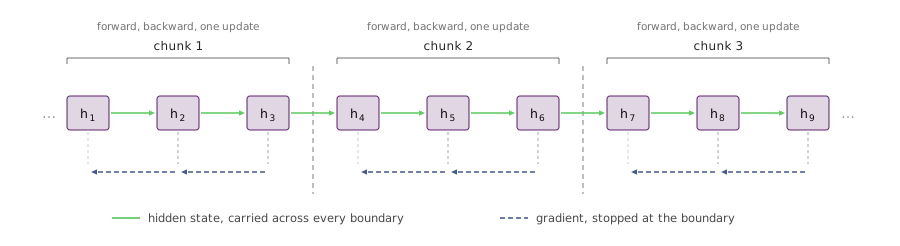
The cost is specific and worth stating plainly rather than filing under “approximation”. A dependency that spans more steps than the chunk length is not learned poorly; it is not learned at all. If the chunk is forty steps and the answer at step 100 depends on something at step 20, no gradient ever connects them, and no amount of training will make the model use that connection. Truncation does not blur long-range dependencies, it deletes the gradient signal for them, and the model retains only whatever such structure it can pick up indirectly through the state it inherits.

There is a second, milder cost. Applying an update per chunk rather than one update over the whole sequence means the weights used in chunk three are not the weights that produced the state that chunk three inherited, so the computation being differentiated is not quite the computation that was run. This is the same inconsistency that appears in distributed training, where gradients computed independently on several devices are applied to one set of weights, and it is tolerated for the same reason: the updates are small, and the alternative does not fit in memory.

8.6 One character at a time

The task that makes recurrence pay is deceptively small: given the text so far, predict the next character. Fix a vocabulary — for a worked example take just $\{\texttt{h}, \texttt{e}, \texttt{l}, \texttt{o}\}$ and the training string hello — and the problem becomes aligned many-to-many classification. At each position the model sees one character and must produce a distribution over the vocabulary for the next one, so the input at step $t$ is the character at position $t$ and the target is the character at position $t+1$.

Nothing about that requires a labelled dataset, and this is the property that matters more than any architectural detail in this chapter. The label at every position is simply the next character, which the text already contains. Any body of text is training data for this task the moment it is written down, and the reason language models became what they are is that this removes the annotation bottleneck entirely — the supervision is free, so the only limit is how much text exists.

Mechanically, each character enters as a one-hot vector $x_t \in \mathbb{R}^V$: a single $1$ in the position of that character and zeros elsewhere, where $V$ is the vocabulary size. The product $W_{xh}x_t$ then selects one column of $W_{xh}$ and discards the rest, which means the matrix multiply is a table lookup written as arithmetic. Implementations do the lookup directly instead, and the matrix is called an embedding — a learned $D$-dimensional vector per vocabulary entry, held in a $D \times V$ table. Two things are gained. The multiply is skipped, which matters when $V$ is in the tens of thousands. More interestingly, since the vectors are learned, characters or words that behave alike come to sit near one another, so the model is handed a representation with structure rather than $V$ mutually orthogonal symbols with none.

Out the other end, $y_t$ is a vector of $V$ scores, one per vocabulary entry, turned into a distribution by the softmax of Section 3.6 and scored by the cross-entropy of the same section:

$$p_t = \operatorname{softmax}(y_t), \qquad L_t = -\log p_t\!\left[x_{t+1}\right], \tag{8.10}$$

with $p_t[x_{t+1}]$ the probability the model assigned to the character that actually came next. The total loss over the sequence is Equation 8.9. There is no new machinery here at all: a character-level language model is a $V$-way classifier applied once per position, and the recurrence is what lets the classifier at position $t$ see everything before it.

Generation is where the model stops resembling a classifier. Feed it a starting character, read the distribution it produces, choose a character from that distribution, feed that choice back in as the next input, and repeat. The loop terminates when the model emits a designated end-of-sequence token, which is why vocabularies carry <START> and <END> entries that correspond to no actual character.

The choice at each step is worth dwelling on, because taking the most probable character — greedy decoding — is both the obvious thing to do and usually wrong. A model with fixed weights and a fixed starting character will make the same greedy choice every time, so it produces exactly one output sequence, forever. Sampling from the distribution instead makes generation stochastic, and it also stops the model from committing to a locally attractive character that leads somewhere with no good continuation. That greedy decoding can be beaten by taking a less likely character now is the entire premise of beam search, which keeps several candidate sequences alive and scores them by the probability of the whole sequence rather than of the next symbol. How to sample from a language model remains an active research question and is not settled by anything in this chapter.

One asymmetry between training and generation is easy to miss and has a name. During training, the input at step $t$ is the true character from the corpus, regardless of what the model predicted at step $t-1$; during generation, the input at step $t$ is whatever the model itself produced. The first is teacher forcing, and it is what makes training parallel over positions within a chunk and stable early on, when the model’s own output is noise. But it means the model is only ever trained on inputs drawn from real text, and at generation time it is asked to continue from its own output — which, after a mistake, is text no corpus would contain. The model has no experience of recovering from its own errors because it was never allowed to make any. This mismatch is called exposure bias, and it is why a generated passage often drifts: each small error moves the input further from anything seen in training, which makes the next error more likely.

8.7 What the state ends up holding

Train the model of Section 8.6 on Shakespeare and watch the samples as training proceeds. Early on they are gibberish — the weights are near their initialization and the distribution is close to uniform over the vocabulary. Some way in, the character statistics arrive: the output has the letter frequencies of English, plausible-looking non-words, and spaces in roughly the right places. Later still it produces real words, then correct spelling and punctuation, then the layout of a play — a name on its own line, a colon, an indented speech. All of it from a model that has only ever been asked what character comes next, and that has been told nothing about words, let alone about speakers.

Train it on the Linux kernel source instead and the same thing happens in a different key. The output is C that would not compile but reads at a glance as C: braces open and close in matched pairs, indentation tracks nesting depth, comments begin with /* and end with */, function definitions are followed by bodies. Syntax is a long-range constraint — a brace opened forty characters ago has to be closed — and the model is learning it from nothing but character co-occurrence.

The line from those experiments to current practice is short and worth stating without the mythology. Today’s coding assistants are trained on the same objective on the same kind of data; what changed is that the unit of prediction became a token rather than a character, the architecture became the one Section 8.12 points toward, and the corpus and the compute grew by many orders of magnitude. The task did not change.

Because a hidden state is just a vector, one can take a single coordinate of it, run the model over a passage, and colour each character by that coordinate’s value. Doing this systematically (Karpathy, Johnson and Fei-Fei, 2015) turns up cells with legible jobs. One switches on at an opening quotation mark and off at the closing one, holding a value across everything between — the model has allocated a coordinate to remembering that a quote is open, because it needs to know when a closing mark is due. Another decays steadily from the start of a line towards where a newline is likely, functioning as a position counter. In the code model there is a cell active inside if statements, a cell active inside comment blocks, and one whose value rises with each level of indentation and falls on the way back out.

This is a genuinely strong result and it is routinely overstated, so two qualifications belong with it. The first is that nobody specified those cells. There is no term in Equation 8.10 mentioning quotation marks; the pressure to predict the next character was sufficient, and the mechanism the network found is recognisably the one the hand-built network of Section 8.3 used — a coordinate reserved to carry one fact forward. The second is that most cells are not like this. Scan the hidden state and the large majority of coordinates produce colourings that look like noise, carrying distributed fragments of many quantities at once and corresponding to nothing nameable. The interpretable cells are the exception that got published, and reading them as evidence that the state decomposes into human-legible variables is reading too much into a favourable sample.

8.8 One network’s output as another’s input

Captioning is the one-to-many shape and the first place in these notes where two networks of different kinds are joined. The recipe follows directly from Section 7.12: take a convolutional network trained on ImageNet, discard the final classification layer, and keep the vector the penultimate layer produces. That vector is not a set of class scores — it is a description of the image in a few thousand dimensions, and it is exactly what the recurrent model needs to be told about.

The join is a third term in the recurrence. Writing $v$ for the image vector, every step computes

$$h_t = \tanh\!\left(W_{hh}\,h_{t-1} + W_{xh}\,x_t + W_{ih}\,v\right), \tag{8.11}$$

with $W_{ih}$ a new learned matrix mapping the image into the hidden space. Note that $v$ carries no subscript: the same image vector is supplied at every step, so the image conditions the whole sentence rather than only its beginning. The alternative, using $v$ to initialize $h_0$ and letting it fade thereafter, is also in use and is the weaker of the two for the obvious reason.

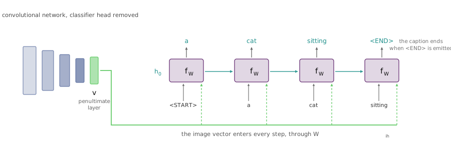
Figure 8.4: Captioning as two networks joined at a vector. The convolutional stack runs once and its penultimate layer, rather than its class scores, becomes the image vector $v$; $v$ then enters every step of the recurrence through $W_{ih}$, alongside the previous hidden state and the previously emitted word. Generation starts from <START> and ends when the model emits <END>, which is what allows the caption to be of a length the model chooses. Drawn for these notes.

The input at each step is the previous word, as Section 8.4 anticipated, which makes the caption autoregressive: the model conditions on the image and on what it has said so far. The sequence starts from a <START> token, and it stops when the model emits <END> — a token that exists only so that the model can decide how long the caption should be, which is the whole point of the one-to-many shape.

These models worked, and their outputs from around 2015 (Karpathy and Fei-Fei; Vinyals et al.) still read as surprising: a cat sitting on a suitcase, a man riding a dirt bike on a dirt track. The failures are more instructive than the successes, because they fail in one characteristic way. A hand held palm-up around a flat object becomes “a person holding a computer mouse”. A woman in a fur coat becomes a woman holding a cat. A person standing on a beach acquires a surfboard they are not carrying. A baseball player with a glove raised to receive a ball is described as throwing one.

Each of these substitutes what is common for what is present. The training objective in Equation 8.10 rewards the caption the corpus would most plausibly contain given this image, and in a corpus of captioned photographs beaches co-occur with surfboards, so a beach raises the probability of the word regardless of whether the object is in the frame. The model is not misperceiving the surfboard; it never needed to perceive one, because predicting it was the better bet. Nothing in the training signal distinguishes reporting from guessing, and so nothing forces the model to learn the difference. This is the same failure that vision-language models are still called out for a decade later, under the name hallucination, and its cause has not changed.

Two variations on the same join produce two further tasks. Feed the model a question alongside the image and score candidate answers and you have visual question answering; keep the dialogue history in the state and the model can be asked follow-up questions about the same image. Feed it an instruction and a stream of images that changes as it moves, and have it emit actions rather than words, and it becomes a navigation agent. At the time these were separate research problems with separate architectures; the observation worth carrying forward is that all of them are Equation 8.11 with a different choice of what conditions the recurrence and what the outputs are scored against.

8.9 Depth in the other direction

Everything so far has used one recurrent layer, and there is no reason to. Stacking gives a grid: the hidden states run along one axis in time and along the other in depth, with layer $\ell$ at step $t$ taking its own previous state $h_{t-1}^{(\ell)}$ and the output of layer $\ell-1$ at the same step. The first layer reads the actual input; each layer above reads what the layer below produced. Recurrence stays within a layer — layer 2’s state never depends directly on layer 1’s state at an earlier step — and the vertical connections carry only the current step.

This helps, and it helps much less than depth helped in Section 7.5. Two or three layers is standard, four is unusual, and there is no recurrent counterpart to the hundred-layer networks of the previous chapter. The reason is that the unrolled graph is already deep: a sequence of length $T$ puts $T$ nonlinearities between the first input and the last output, so a two-layer network on a sequence of length 100 is differentiating through a graph of depth 200. Adding layers multiplies a depth that was never the scarce resource. Whatever limits an RNN, it is not that the computation between input and output is too shallow — which is precisely what Section 8.10 is about.

8.10 Why the gradient dies

Everything good about the recurrence comes from applying one function repeatedly. Everything wrong with it comes from the same place, and the mechanism is visible in a single derivative. Differentiating Equation 8.3 with respect to the state it consumed gives

$$\frac{\partial h_t}{\partial h_{t-1}} = \operatorname{diag}\!\left(\tanh'\!\left(W_{hh}h_{t-1} + W_{xh}x_t\right)\right) W_{hh}, \tag{8.12}$$

a diagonal matrix of activation derivatives multiplied by $W_{hh}$. Gradients flowing from step $T$ back to step $k$ pass through one such factor per step, and the chain rule multiplies them:

$$\frac{\partial h_T}{\partial h_k} = \prod_{t=k+1}^{T} \frac{\partial h_t}{\partial h_{t-1}} . \tag{8.13}$$

A product of $T-k$ matrices, every one of which contains the same $W_{hh}$. That is the whole problem, and it is a problem about repeated multiplication rather than about sequences.

To see what repeated multiplication does, delete the nonlinearity for a moment and suppose $\tanh'$ were identically $1$. Then Equation 8.13 is $W_{hh}$ raised to the power $T-k$, and the behaviour of a matrix power is governed by its largest singular value $\sigma_1$ — the most a unit vector can be stretched by one application. If $\sigma_1 > 1$, the norm grows geometrically and the gradient explodes. If $\sigma_1 < 1$, it shrinks geometrically and the gradient vanishes. Only $\sigma_1$ exactly equal to $1$ is stable, and that is a knife edge no training procedure will balance on. There is no benign regime; a matrix applied a hundred times either amplifies or annihilates.

Figure 8.5: What repeated multiplication does to a gradient. Each curve is the norm of a vector after $k$ applications of a matrix with the largest singular value marked, on a logarithmic scale, so geometric growth and decay both appear as straight lines. At $\sigma_1 = 1.05$ the gradient is a thousand times its original size after 150 steps; at $\sigma_1 = 0.95$ it is a thousandth. The dashed curve adds the effect of $\tanh'$, whose value never exceeds $1$ and is typically well below it: even the expanding matrix now decays. Nothing in the vanilla recurrence puts a curve near the horizontal. Computed for these notes.

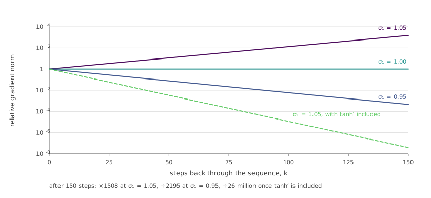
Restoring the nonlinearity breaks the symmetry, and not in the helpful direction. The derivative of $\tanh$ is at most $1$, attained only at the origin, and falls away sharply on either side; any state that is not near zero contributes a factor well below $1$. So the diagonal in Equation 8.12 scales the product down at every step, which drags even a $W_{hh}$ with $\sigma_1$ slightly above $1$ toward collapse. The property that made $\tanh$ attractive in Section 8.2 — that it keeps the forward state bounded — is exactly the property that starves the backward pass, and this tension is not resolvable by choosing a different bounded activation.

The two failures are not equally serious, which is worth being precise about because they are usually named as a matched pair. Explosion is loud and has a crude, effective fix. When the gradient’s norm exceeds a threshold $\theta$, rescale it:

$$g \leftarrow \frac{\theta}{\lVert g \rVert}\, g \qquad \text{whenever } \lVert g \rVert > \theta . \tag{8.14}$$

Gradient clipping (Pascanu, Mikolov and Bengio, 2013) keeps the direction and discards the magnitude, which is a defensible trade because a gradient of norm $10^6$ was never a trustworthy step length in the first place. It is a one-line change and it works.

Vanishing has no such fix, and the reason is not that the gradient is small. Rescaling a small gradient upwards is easy; the difficulty is that Equation 8.8 sums contributions from every step, and the contributions from distant steps have decayed by a factor of $\sigma_1^{T-k}$ relative to those from nearby ones. The total gradient is therefore not small — it is dominated by short-range dependencies, and the long-range signal is buried underneath them. Multiplying the sum by any constant multiplies both parts equally. The information about long-range structure has not been attenuated so much as overwritten, and it is unrecoverable after the fact.

That is why the honest conclusion is architectural rather than algorithmic. Learning long-range dependencies with a vanilla RNN would require $W_{hh}$ to be, and to remain throughout training, a matrix whose repeated application neither grows nor shrinks its input — while also being the matrix that does the model’s actual computational work. Those two demands are in direct conflict, and asking one matrix to satisfy both is the design error. The fix is to change the recurrence so that some path from $h_{t-1}$ to $h_t$ does not pass through a matrix multiply at all.

8.11 LSTM

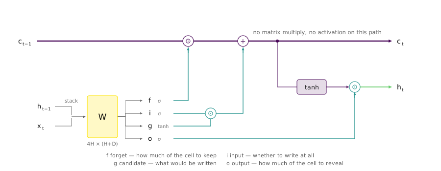
The change was proposed in 1997, well before anything in this chapter had a use for it (Hochreiter and Schmidhuber), and it consists of carrying two vectors between steps instead of one. The cell state $c_t$ is the long-term memory and is not exposed outside the layer; the hidden state $h_t$ is what the rest of the network sees. The point of the split is that the two can be updated by different mechanisms, and the cell’s is chosen so that a gradient can travel along it undamaged.

One matrix multiply produces four vectors at once. Stack the previous hidden state and the current input, multiply by a single $W$ of shape $4H \times (H + D)$, and split the $4H$-dimensional result into four blocks of size $H$:

$$\begin{pmatrix} i \\ f \\ o \\ g \end{pmatrix} = \begin{pmatrix} \sigma \\ \sigma \\ \sigma \\ \tanh \end{pmatrix} W \begin{pmatrix} h_{t-1} \\ x_t \end{pmatrix}. \tag{8.15}$$

Three blocks pass through a sigmoid and so lie in $(0,1)$; these are the gates, and a value near $0$ closes and near $1$ opens. The fourth passes through $\tanh$ and lies in $(-1,1)$; it is candidate content rather than a gate. Their jobs: $f$, the forget gate, decides how much of the existing cell to keep; $i$, the input gate, decides whether to write at all; $g$ is what would be written; and $o$, the output gate, decides how much of the cell to expose. The stacking is a matter of implementation — four matrices concatenated into one so a single multiply computes all four — and the shapes above are what makes an LSTM roughly four times the parameters of a vanilla RNN with the same hidden size.

The state updates are two lines, and the first is the one that matters:

$$c_t = f \odot c_{t-1} + i \odot g, \qquad h_t = o \odot \tanh(c_t), \tag{8.16}$$

where $\odot$ is elementwise multiplication. Read Equation 8.16 as an instruction about memory: erase part of what is stored, scaled by $f$; write new content $g$, scaled by $i$; then reveal some fraction of the result, scaled by $o$. Each coordinate of the cell is governed independently, so the layer can hold one quantity untouched for hundreds of steps while rewriting another every step.

Figure 8.6: One LSTM step. The cell state runs along the top and is modified only by an elementwise multiply with the forget gate and an addition of the gated candidate — no matrix multiply, no activation function stands on it. Everything below computes the four gates from one product of $W$ with the stacked previous hidden state and current input. The hidden state that leaves on the right is a gated, squashed view of the cell, and is what the rest of the network sees. Drawn for these notes.

Now differentiate the cell update, which is the entire argument:

$$\frac{\partial c_t}{\partial c_{t-1}} = \operatorname{diag}(f). \tag{8.17}$$

Compare it with Equation 8.12. There is no $W_{hh}$ in it and no $\tanh'$ in it. A gradient travelling backwards along the cell state is multiplied by the forget gate and by nothing else, so the product in Equation 8.13 becomes a product of forget gates rather than a matrix power. The path along the top of Figure 8.6 is an uninterrupted channel from the end of the sequence to the beginning.

This is the residual connection of Section 7.8, arrived at independently and eighteen years earlier. With $f$ near $1$ the update reads $c_t \approx c_{t-1} + i \odot g$: a quantity carried forward unchanged plus a correction, which is Equation 7.9 with time in place of depth. The two mechanisms answer the same question — how does a signal cross many stages of processing without being destroyed — and both answer it by providing a route that skips the processing. The difference is what the stages are. ResNet stacks layers; the LSTM stacks time steps, and unlike layers, their number is set by the data.

Whether this solves vanishing gradients is the question the lecture asks and answers carefully, and the careful answer is no. The forget gate is a sigmoid, so $f < 1$ strictly, and a product of many numbers below $1$ still decays. What has changed is who chooses. In a vanilla RNN the decay rate is a property of $W_{hh}$, one number for the whole model, applied identically to every coordinate and every step, and set by whatever the optimizer happened to need for the model’s other work. In an LSTM the decay is per coordinate and per step, computed from the data, and learnable — so the network can drive $f$ toward $1$ on the coordinates holding something it will need later and toward $0$ on the ones it wants to clear, and it can make that decision differently at different points in the sequence. Preserving information across a hundred steps went from something the model must arrange as a side effect of a single shared matrix to something it can simply ask for. The LSTM does not remove the mathematics of Section 8.10; it hands the model the controls.

8.12 What recurrence costs

Set the gradient problem aside for a moment and look at what the recurrence buys and what it charges, because the ledger is what determines the next chapter.

On the credit side, the model has no maximum input length. The state is the same size at step 10 and step 10 million, so the parameter count does not depend on how long the sequence is and there is no architectural quantity that has to be chosen in advance and then lived with. Compute grows linearly with the sequence: doubling the input doubles the work, exactly. Nothing about the model needs to be told the sequence length before it runs.

On the debit side, two things, and both are structural rather than incidental. The first is the bottleneck. Everything the model knows about the past is compressed into one fixed-size vector, and a vector of a thousand dimensions is the whole of the model’s memory whether the sequence has been ten steps or a hundred thousand. Something must be discarded, and no amount of gating changes that — the LSTM improves how well the model can choose what to keep, not how much it can keep.

The second is sequential dependency, and it is the more damaging of the two in practice. Step $t$ cannot begin until step $t-1$ has finished, because it consumes $h_{t-1}$. The sequence dimension therefore does not parallelize, and the depth of the critical path in the computation is the length of the input. This is tolerable at generation time, where any autoregressive model must produce one symbol before the next regardless of architecture, but it is severe during training, where the targets at every position are known in advance and could in principle all be processed at once. A model that cannot exploit that cannot use a modern accelerator well, and cannot be scaled by throwing hardware at it — which, over the following decade, was how essentially all progress happened.

Both debits are removed by the mechanism of the next chapter, and it is worth saying now what it costs to remove them, because the trade is not free. Attention lets every position look directly at every other, so there is no fixed-size summary to squeeze through and no chain of dependencies to serialize; a whole training sequence is processed in one parallel operation. The price is that comparing every position with every other is quadratic in the sequence length, where the RNN was linear, and that the set of positions attended to must be bounded in advance — the context window that recurrent models do not have.

Which is why the recurrent idea has come back rather than expired. A line of recent work — Mamba, RWKV and the broader family of state space models — keeps the recurrent form, a state carried forward and updated in linear time with no context limit, while restructuring the update so that training can still be parallelized across the sequence. The equations look nothing like Equation 8.3, but the shape of the answer is the one this chapter has been describing: a fixed-size state, carried forward, rewritten at every step.

8.13 What this leaves

The chapter began with a shape problem — a network that fixes its input and output sizes cannot caption an image or classify a video — and answered it with one line, Equation 8.1, applied over and over. Everything else followed from that repetition. Unrolling made the model differentiable with machinery already built; sharing $W$ across steps made it length-agnostic and made the gradient a sum; truncation made it fit in memory at the cost of long-range signal; and the repeated multiplication in Equation 8.13 made long-range learning hard in a way no choice of hyperparameter fixes. The LSTM is a direct answer to that last consequence and to nothing else.

What deserves to be carried forward is not the vanilla RNN, which is rarely the right choice today, but three things that outlived it. The first is that a shared weight used $T$ times contributes $T$ gradients that are summed — a fact about graphs, not about sequences, and one that reappears everywhere parameters are reused. The second is the additive path: whenever a signal must survive many stages, give it a route that skips them, which is the LSTM cell and the residual connection and the same idea twice. The third is the language-modelling objective of Section 8.6, which asks only for the next symbol, needs no labels, and turned out to be enough to induce syntax, structure, and rather more.

The next chapter takes up what Section 8.12 left open. If the difficulty is that information from step 5 must survive 500 sequential rewrites to be available at step 505, the sharper question is why it should have to travel through them at all.

References

• Y. Bengio, P. Simard and P. Frasconi, “Learning Long-Term Dependencies with Gradient Descent Is Difficult,” IEEE Transactions on Neural Networks 5(2):157–166, 1994. DOI
• J. L. Elman, “Finding Structure in Time,” Cognitive Science 14(2):179–211, 1990. DOI
• A. Gu and T. Dao, “Mamba: Linear-Time Sequence Modeling with Selective State Spaces,” 2023. arXiv:2312.00752
• S. Hochreiter and J. Schmidhuber, “Long Short-Term Memory,” Neural Computation 9(8):1735–1780, 1997. DOI
• A. Karpathy, J. Johnson and L. Fei-Fei, “Visualizing and Understanding Recurrent Networks,” 2015. arXiv:1506.02078
• A. Karpathy and L. Fei-Fei, “Deep Visual-Semantic Alignments for Generating Image Descriptions,” CVPR, 2015. Paper
• R. Pascanu, T. Mikolov and Y. Bengio, “On the Difficulty of Training Recurrent Neural Networks,” ICML, 2013. arXiv:1211.5063
• B. Peng et al., “RWKV: Reinventing RNNs for the Transformer Era,” EMNLP Findings, 2023. arXiv:2305.13048
• O. Vinyals, A. Toshev, S. Bengio and D. Erhan, “Show and Tell: A Neural Image Caption Generator,” CVPR, 2015. arXiv:1411.4555
• S. Antol et al., “VQA: Visual Question Answering,” ICCV, 2015. arXiv:1505.00468