5  Neural Networks and Backpropagation

Lecture 4

Based on Lecture 4 of CS231n, Stanford University, Spring 2025.

5.1 What the hidden layer buys

Equation 4.18 arrived at the end of the previous chapter as a repair. The linear model could not represent what the data required, so the proposal was to learn the representation rather than choose it. That says what the extra layer is for without saying what it does, and the difference is worth making concrete, because it is visible in the shapes alone.

Take CIFAR-10, where an image is $D = 3072$ numbers and there are $C = 10$ classes. The linear model of Equation 3.4 has a single matrix of shape $10 \times 3072$. The two-layer model splits that into $W_1$ of shape $100 \times 3072$ and $W_2$ of shape $10 \times 100$, with the hidden vector $h = \max(0, W_1 x)$ carrying a hundred numbers between them. Nothing has been added to the input and nothing has been added to the output; the model has simply been made to pass its evidence through a hundred-dimensional bottleneck of its own design.

The consequence follows from what a row of a weight matrix can do. As Section 3.4 put it, each row of $W$ scores an image by correlating it with a fixed pattern, so the ten rows are ten templates and the classification is a contest between them. A single row for horse has to respond to every horse in the training set. Horses photographed facing left put bright pixels where horses facing right put background, and one row that scores both of them highly is a compromise between the two—which is why the learned template, viewed as an image, tends to show an animal with a head at each end. That is not a failure of the optimizer. It is the best that one template can do when the class it describes appears in incompatible configurations.

The hundred rows of $W_1$ are under no such obligation, because none of them is required to correspond to a class. One row is free to respond to a left-facing horse and another to a right-facing one, and the horse row of $W_2$ can weight both positively, so the two poses are recognised separately and then added rather than averaged into one. The same freedom cuts the other way: a hidden unit that responds to a dark round region surrounded by lighter pixels is useful to bird, cat, deer, dog and horse at once, and every one of those output rows can draw on it. The hidden layer holds features that classes share; the output layer holds the part that is specific to a class. A hundred templates instead of ten, and reuse between them, is the entire structural gain.

Depth extends the same move rather than introducing a new one. A three-layer network,

$$f(x, W_1, W_2, W_3) = W_3 \max(0, W_2 \max(0, W_1 x)), \tag{5.1}$$

lets the second hidden layer build its features from the first layer’s features instead of from raw pixels, so that a unit can respond to a configuration of parts rather than to a pattern of pixels. The dimensions have to agree along the chain and nothing else constrains them. In practice each layer also carries a learnable bias, written $W_1 x + b_1$, which is omitted here only to keep the composition readable.

The naming convention is a persistent source of confusion and is worth stating once. A network is counted by its weight matrices, not by its non-linearities: Equation 4.18 is a two-layer network with one hidden layer, and Equation 5.1 is a three-layer network with two hidden layers. Layers of this kind, in which every input to a layer influences every output of it, are called fully connected layers, and networks built from them are fully connected networks or multi-layer perceptrons—both more precise than “neural network”, which names a family far larger than this.

Figure 5.1: Two fully connected networks drawn as graphs. Left: one hidden layer, so two weight matrices and a two-layer network. Right: two hidden layers and three weight matrices. Every unit in a layer is connected to every unit in the next, which is what “fully connected” names; the arrows carry the weights and the layers carry the activations. Drawn for these notes.

5.2 What the max is doing

The previous chapter observed that removing the $\max$ from Equation 4.18 collapses $W_2 W_1$ into a single matrix and returns the model to a linear classifier. That is a proof that the non-linearity is necessary. It is not an account of what the non-linearity contributes, and the account turns out to be simple enough to see in one dimension.

Consider a single hidden unit reading a scalar input, computing $\max(0, wx + b)$. Its output is zero for every $x$ on one side of the point $x = -b/w$ and rises linearly on the other. The unit is two straight pieces joined at a corner, and the position of that corner is set by $b/w$—which is to say, by the parameters, which is to say, by training. A weighted sum of $H$ such units is again made of straight pieces, with at most $H$ corners, each placed where one unit switches on.

This is what the network’s capacity to fit a curve consists of. A two-layer network with a ReLU non-linearity computes a piecewise-linear function, gradient descent adjusts both the slopes of the pieces and the locations of the joints between them, and the number of joints available is bounded by the width of the hidden layer. Fitting a smooth function means approximating it by a polyline whose vertices the optimizer is free to move, which is why width buys accuracy and why the approximation is exact nowhere and adequate everywhere.

Figure 5.2: A weighted sum of three ReLU units, each contributing one corner. The three units are drawn beneath the axis they act on, with the location of each corner set by that unit’s own weight and bias; their weighted sum, above, is the piecewise-linear function the network computes. Adding units adds corners, which is the sense in which width buys the ability to fit a curve. Drawn for these notes.

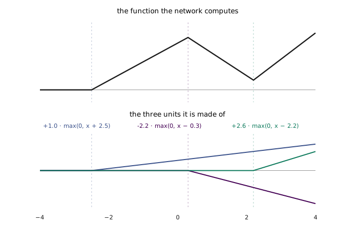
In $D$ dimensions the picture is the same with the corners replaced by hyperplanes. Each hidden unit divides input space in two along the plane where its pre-activation crosses zero, the units together cut the space into regions, and within any one region the set of active units is fixed, so the network is exactly affine there. The network is a collection of linear models with a learned rule for choosing between them. Depth matters here in a way width does not, because a second hidden layer folds the regions produced by the first, and the number of distinct regions available grows much faster with depth than with width (Montúfar et al., 2014).

One detail of this construction matters later. A piecewise-linear function is not differentiable at its corners, so $\max(0, z)$ has no derivative at $z = 0$, and every framework simply picks a value there—PyTorch returns zero. The choice is arbitrary and inconsequential, because the set of inputs landing exactly on a corner has measure zero, but it is worth knowing that it was made rather than derived.

5.3 Choosing an activation

The rectified linear unit, $\max(0, z)$, is the default and deserves to be. It costs one comparison, it does not saturate for positive inputs, and its derivative is exactly one wherever it is active, so a gradient passing through many layers of ReLU is neither amplified nor attenuated by the activation itself. Every alternative below is an attempt to fix one specific complaint about it, and the complaints are worth understanding because the same failure modes recur throughout the course.

The complaint against ReLU is that a unit can die. If a unit’s pre-activation is negative for every example in the training set, its output is zero for all of them, its derivative is zero for all of them, and no gradient reaches its weights ever again. It is not merely inactive but unrecoverable, and a network can lose a substantial fraction of its units this way, typically to a learning rate large enough to push a whole row of $W_1$ off the data in one step. Leaky ReLU replaces the flat half with a shallow slope,

$$\text{LeakyReLU}(z) = \max(\alpha z, z), \qquad \alpha = 0.01, \tag{5.2}$$

so that a unit with negative pre-activation still passes a small gradient and can be pushed back. The exponential linear unit does the same with a smooth curve that approaches $-\alpha$ instead of falling away linearly, which also brings the mean output nearer zero.

The smooth variants matter for a reason that only shows up in deeper models. The Gaussian error linear unit multiplies the input by the probability that a standard normal variable falls below it,

$$\text{GELU}(z) = z\,\Phi(z), \tag{5.3}$$

giving a function that behaves like ReLU far from the origin but has a continuous derivative and a small negative dip just below zero (Hendrycks and Gimpel, 2016). The sigmoid linear unit, $z\,\sigma(z)$, has the same shape from a different construction. These are the activations used in transformers and in several convolutional families, and the argument for them is empirical rather than principled: the loss surface they produce is easier to descend, and the gain is real but small.

Figure 5.3: Five activation functions on shared axes. ReLU and leaky ReLU coincide exactly for positive inputs and differ only for negative ones; leaky ReLU is drawn here with $\alpha = 0.1$ rather than the $0.01$ of Equation 5.2, because at $0.01$ the negative slope is under half a pixel across the whole plot. GELU tracks ReLU away from the origin but is smooth through it, dipping slightly below zero. Sigmoid and tanh are bounded, and both flatten at each end—the regions where a gradient arriving from above is destroyed. Drawn for these notes.

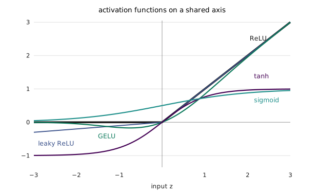
Sigmoid and tanh predate all of these and are now the wrong choice inside a network, for a reason that is quantitative rather than aesthetic. The derivative of $\sigma(z) = 1/(1 + e^{-z})$ is $\sigma(z)\,(1 - \sigma(z))$, which attains its maximum of $0.25$ at $z = 0$ and decays towards zero in both directions. A gradient crossing a sigmoid is therefore multiplied by at most a quarter even under the most favourable conditions, and by very much less once the unit is anywhere near saturation, so ten such layers attenuate the gradient by a factor of at least $4^{10} \approx 10^6$ before it reaches the first weight matrix. This is the vanishing gradient problem in its simplest form, and it is why networks of this depth were not trainable before rectifiers.

Sigmoid carries a second, subtler defect: its output is always positive. Every input to the next layer is therefore positive, and by the local-gradient rule developed in Section 5.10, that forces every element of the gradient with respect to a row of the next weight matrix to carry the same sign. The row can only move up in all coordinates or down in all coordinates, so a direction requiring one weight to rise and another to fall must be reached by a zigzag—exactly the poorly conditioned descent of Section 4.7, produced here by the activation rather than by the data. Tanh, being $2\sigma(2z) - 1$, fixes the centring and raises the maximum derivative to one, which makes it strictly better than sigmoid as a hidden activation while leaving the saturation intact.

Both still have a use at the output, where saturation is the point rather than the problem: a sigmoid maps a score to a probability for a binary decision, and tanh maps one to a bounded quantity. Inside the network, the practical advice is what the empirical record supports. Use ReLU unless the architecture family you are working in has an established alternative, in which case use that one, and treat the choice as a hyperparameter to be validated rather than a question with a general answer.

5.4 Depth, width and the forward pass

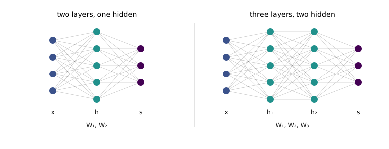
Evaluating Equation 4.18 is a matrix product, an elementwise maximum, and a second matrix product. Nothing in it is expensive to state and nothing in it is expensive to run, which is the reason this particular model became the default unit of construction rather than any of the more biologically motivated alternatives: it is exactly the operation that a GPU executes fastest. The regularity of a fully connected layer—every input reaching every output, in one dense matrix—is a decision about hardware as much as about modelling.

The forward pass over a batch is worth writing with its shapes attached, because in an implementation the shapes are what you debug. With $N$ examples stacked as rows, the input is a matrix $x$ of shape $N \times D$, the first weight matrix is $D \times H$, and the hidden activations $h = \max(0, xW_1)$ come out $N \times H$; the second weight matrix is $H \times C$ and the scores are $N \times C$. Every example travels through independently and the batch dimension is carried along untouched, which is why a batch of any size works without changing a line.

Training the whole thing is that forward pass, the gradient of the loss with respect to each weight matrix, and the update from Equation 4.5. In a numerical library it fits in twenty lines with nothing hidden:

import numpy as np

N, D_in, H, D_out = 64, 1000, 100, 10
x, y = np.random.randn(N, D_in), np.random.randn(N, D_out)
w1 = np.random.randn(D_in, H) / np.sqrt(D_in)
w2 = np.random.randn(H, D_out) / np.sqrt(H)

for t in range(2000):
    h = np.maximum(0, x.dot(w1))          # forward: hidden activations
    y_pred = h.dot(w2)                    # forward: scores
    loss = np.square(y_pred - y).sum()    # forward: squared error

    grad_y_pred = 2.0 * (y_pred - y)      # backward: through the loss
    grad_w2 = h.T.dot(grad_y_pred)
    grad_h = grad_y_pred.dot(w2.T)
    grad_h[h <= 0] = 0                    # backward: through the ReLU
    grad_w1 = x.T.dot(grad_h)

    w1 -= 1e-4 * grad_w1                  # gradient descent
    w2 -= 1e-4 * grad_w2

Two details in that listing are not decoration. The weight matrices are divided by the square root of their input dimension, because drawing them from a unit normal would give a pre-activation with standard deviation $\sqrt{1000} \approx 31.6$ and a first loss large enough to diverge at any usable learning rate; initialization is a subject in its own right and this is the crudest form of the fix. And the line grad_h[h <= 0] = 0 is the backward pass of the $\max$—a gradient reaches a hidden unit only where that unit was active going forwards. Everything else is the chain rule applied by hand, which is precisely the thing that will not survive the next section.

Run it and the loss falls from $862$ to under $10^{-3}$ within two hundred steps and to zero shortly after. That is not a good result; it is the point of the next section. The targets y are random numbers, so there is nothing to learn, and a hundred hidden units have simply memorised sixty-four arbitrary vectors.

5.5 Size is not a regularizer

More units mean more capacity, and more capacity means a decision boundary that can wander further to accommodate individual training points. The shape of the failure is familiar from Section 3.2: a one-nearest-neighbour classifier carves an island around every noisy example, and a wide network does the same thing with a smooth boundary instead of a Voronoi cell. Faced with a model that fits the training set and fails on held-out data, the obvious repair is to build a smaller one.

The advice is to resist it, and the reason is not that smaller networks generalise badly. It is that width and regularization strength are not interchangeable knobs even when they move the same quantity. The penalty weight $\lambda$ of Equation 4.1 is continuous, so a validation sweep over it explores capacity finely; the width of a layer is an integer that changes the model’s architecture, its initialization, its memory footprint and the shape of its loss surface all at once, and a sweep over it is a sweep over different training runs rather than different settings of one run. When a change hurts, $\lambda$ tells you by how much and in which direction. Width tells you much less, at a much higher cost per sample.

The working procedure that follows from this is to grow the network until it is capable of overfitting, and only then to regularize. Overfitting is evidence that the model has enough capacity to represent the structure in the data, which is a prerequisite for learning it; a model that cannot overfit its training set is not being cautious, it is being inadequate, and no amount of tuning $\lambda$ will recover what it cannot represent. Once the model can overfit, $\lambda$ is the instrument that decides how much of that capacity is spent on structure and how much on noise.

That instrument has two ends. Too little regularization gives the boundary in the previous paragraph. Too much constrains the weights so severely that the boundary loses the detail it needed, and the model underfits—the classifier is now failing for the opposite reason and the validation curve looks similar from a distance. Neither end is a subtle effect and both are visible in a sweep, which is exactly the argument for sweeping the quantity that is cheap to sweep.

None of this settles how wide to make the network in the first place, and there is no principled answer. The practice is to start from a width that has worked for similar data and a similar problem, and to explore around it. Recognising which established architecture the problem resembles is a more useful skill than any formula for choosing a layer size, and most of the rest of this course is a tour of those architectures.

5.6 The brain analogy and its limits

The vocabulary comes from biology and the resemblance is real but shallow. A biological neuron collects electrical impulses from many upstream cells through its dendrites, integrates them in the cell body, and emits a signal down its axon when the accumulated input is sufficient. Written as arithmetic, that is a weighted sum followed by a threshold, which is one unit of Equation 4.18 with the activation function playing the part of the threshold. The analogy earned the field its name and is a fair description of where the idea came from.

It is a poor description of what either system is. A cortical neuron is not a scalar rate: it has spike timing, dozens of morphological types, dendrites that themselves compute non-linearly, and neuromodulatory state that changes its behaviour wholesale. Nothing in the brain corresponds to a global scalar loss differentiated back through every synapse, and the layered, densely connected regularity of the models in this chapter was chosen because it maps onto a matrix multiply, not because it maps onto cortex. Networks with irregular connectivity have been built and studied; they perform about as well and are much harder to run, which is the honest reason they are not used. Take the analogy as etymology rather than as evidence.

5.7 Why gradients need a system

Return to the four gradient lines in Section 5.4. They are correct, and they were obtained by differentiating a specific composition—squared error, on top of a linear map, on top of a rectifier, on top of a linear map—once, by hand, on paper. Every part of that sentence is a liability.

Change the loss from squared error to the softmax objective of Equation 3.7 and grad_y_pred is wrong and every line below it inherits the error. Insert a third layer and the derivation restarts. Replace the rectifier and the masking line changes shape. The work is proportional to the architecture, it has to be redone whenever any part of the architecture moves, and it is done in the one place where a mistake is hardest to notice—a gradient that is wrong by a constant factor still trains, slowly and to a worse optimum, and looks like a badly chosen learning rate. Chapter 3’s numerical gradient check exists precisely because this failure is silent.

Tedium is the mild version of the objection. The severe one is that hand differentiation does not scale past architectures you can hold in your head. A recurrent model unrolled over a hundred timesteps, or a network with branches that merge, or anything with a memory that is read and written—the differentiation is not tedious for these, it is infeasible, and the field would have stopped at two layers if it had depended on doing it.

The fix is to stop treating the model as one large formula. Write it instead as a graph in which each node performs a single primitive operation—an addition, a multiplication, a maximum, an exponential—and each edge carries a value from the node that produced it to the nodes that consume it. The inputs to the graph are the data and the parameters; the single output is the scalar loss. Nothing about the model has changed; it has only been decomposed to a granularity at which every individual derivative is something you already know.

What makes the decomposition pay is that the chain rule is local. To send a gradient through a node, that node needs the derivative of its own output with respect to its own inputs, and the gradient of the loss with respect to its output. It needs to know nothing whatsoever about the rest of the graph—not what produced its inputs, not what consumes its outputs, not what loss is being minimised. So if every primitive knows how to differentiate itself, the gradient with respect to every parameter in the graph can be assembled by traversing the graph backwards, once. That procedure is backpropagation.

5.8 The chain rule on a graph

The procedure is easiest to trust after watching it work on something small enough to check by hand. Take

$$f(x, y, z) = (x + y)\,z, \tag{5.4}$$

evaluated at $x = -2$, $y = 5$, $z = -4$. As a graph it has two nodes: an addition consuming $x$ and $y$ and producing an intermediate value $q = x + y$, and a multiplication consuming $q$ and $z$ and producing $f$. The forward pass evaluates them in order, giving $q = 3$ and $f = -12$, and each node keeps its inputs, because the backward pass will need them.

What is wanted is $\partial f/\partial x$, $\partial f/\partial y$ and $\partial f/\partial z$. Two of the four local derivatives are immediate from the addition node, since $q = x + y$ gives $\partial q/\partial x = 1$ and $\partial q/\partial y = 1$. The multiplication node gives the other two: $f = qz$ gives $\partial f/\partial q = z$ and $\partial f/\partial z = q$. Note what those say—the derivative of a product with respect to one factor is the other factor, which is why a multiplication node has to remember both of its inputs.

Now traverse backwards. The gradient of $f$ with respect to itself is $1$. At the multiplication node, the two inputs receive $\partial f/\partial z = q = 3$ and $\partial f/\partial q = z = -4$. At the addition node, the chain rule composes what has arrived from above with what the node contributes locally:

$$\frac{\partial f}{\partial x} = \frac{\partial f}{\partial q}\,\frac{\partial q}{\partial x} = (-4)(1) = -4, \tag{5.5}$$

and identically $\partial f/\partial y = -4$. The results are checkable without any of this machinery: raising $x$ from $-2$ to $-1.99$ raises $q$ to $3.01$ and lowers $f$ to $-12.04$, a change of $-0.04$ for an input change of $0.01$, which is the $-4$ just computed.

Figure 5.4: The graph of Equation 5.4 evaluated at $x=-2$, $y=5$, $z=-4$. Values computed on the forward pass are shown above each edge and gradients of $f$ with respect to that edge below it, in the second colour. The backward pass starts from $\partial f/\partial f = 1$ at the right and moves left, each node multiplying what arrives from above by its own local derivative. Drawn for these notes.

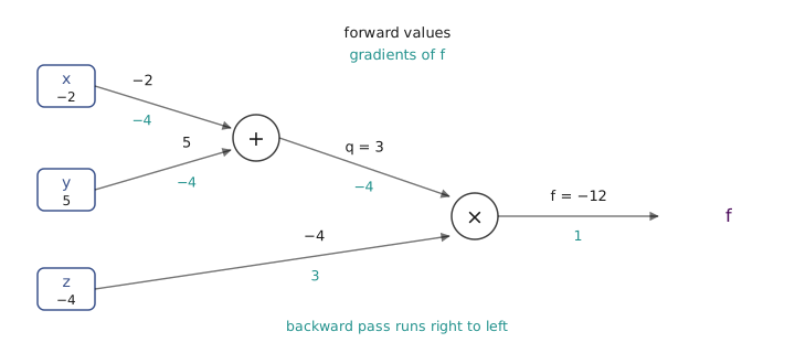
Equation 5.5 is the entire algorithm, and it is worth naming its two factors, because the names are how the rest of this chapter and most framework source code talk about it. The quantity arriving from the node above is the upstream gradient: the derivative of the loss with respect to this node’s output. The derivative the node computes from its own inputs is the local gradient. Their product is the downstream gradient, which the node passes to whatever produced its inputs, where it becomes that node’s upstream gradient in turn.

The recursion terminates because the graph is finite, and it visits each node exactly once, so the whole backward pass costs about what the forward pass costs. This is the property that makes the method viable rather than merely correct. A network with $10^8$ parameters yields all $10^8$ partial derivatives in one traversal, whereas the finite-difference estimate of Section 4.5 would need $10^8$ separate forward passes to get the same information. The asymmetry is not an implementation detail; it is the reason gradient-based learning at this scale exists at all, and it was the point of the paper that introduced the technique to the field (Rumelhart, Hinton and Williams, 1986).

Two things a node emphatically does not need are worth stating, because they are what make the whole scheme composable. It does not need to know what produced its inputs, and it does not need to know what its output feeds into or what loss is eventually computed. It needs its own inputs, its own local derivative, and one number arriving from above.

5.9 A longer example, and a choice about granularity

Take a logistic unit over two inputs,

$$f(w, x) = \frac{1}{1 + \exp\!\left(-(w_0 x_0 + w_1 x_1 + w_2)\right)}, \tag{5.6}$$

at $w_0 = 2$, $x_0 = -1$, $w_1 = -3$, $x_1 = -2$, $w_2 = -3$. Decomposed to primitives the graph runs: two multiplications giving $-2$ and $6$; an addition giving $4$; a second addition with $w_2$ giving $1$; a negation giving $-1$; an exponential giving $0.37$; an addition of one giving $1.37$; and a reciprocal giving $0.73$.

The backward pass walks the same chain in reverse, each step multiplying by one local derivative. The reciprocal $1/u$ has local derivative $-1/u^2 = -1/1.37^2 = -0.53$, so the gradient below it is $-0.53$. Adding a constant has local derivative $1$ and changes nothing. The exponential has local derivative equal to its own output, $0.37$, giving $-0.53 \times 0.37 = -0.20$. The negation flips the sign to $+0.20$. From there the two additions distribute $0.20$ unchanged to $w_2$ and to both products, and each multiplication hands each of its inputs the value of the other scaled by $0.20$: $\partial f/\partial w_0 = x_0 \times 0.20 = -0.20$ and $\partial f/\partial x_0 = w_0 \times 0.20 = 0.40$, and likewise $-0.40$ and $-0.60$ for the second pair.

Eight nodes, eight local derivatives, no step harder than a first-year exercise. But four of those nodes—negate, exponentiate, add one, reciprocate—exist only to compute the logistic function, and the logistic function differentiates in closed form. Writing $\sigma(u) = 1/(1 + e^{-u})$,

$$\frac{d\sigma}{du} = \frac{e^{-u}}{(1 + e^{-u})^2} = \left(\frac{1 + e^{-u} - 1}{1 + e^{-u}}\right)\left(\frac{1}{1 + e^{-u}}\right) = \bigl(1 - \sigma(u)\bigr)\,\sigma(u), \tag{5.7}$$

which at $\sigma = 0.73$ gives $(1 - 0.73)(0.73) = 0.20$—the same number the four-node chain produced, from one multiplication.

So the decomposition into primitives is a choice, not a fact about the function, and the choice is a real engineering trade. A coarse node is faster, because it replaces four kernel launches with one and four cached intermediate tensors with none. It is often numerically better, because a closed form can avoid the cancellations that its own decomposition runs into. And Equation 5.7 has a property worth noticing on its own: the derivative is expressed in terms of the node’s output, so a sigmoid node need not remember its input at all. Against that, every coarse node is a derivative someone has to derive and test by hand, which is the cost the whole method was introduced to avoid. Frameworks resolve this empirically, by writing fused nodes for the operations that are common enough to be worth the effort and leaving everything else composed from primitives.

5.10 Four patterns worth recognising

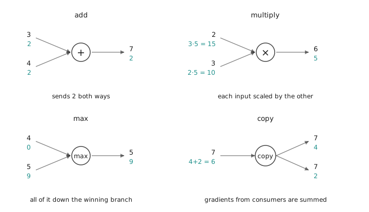
Because the local derivatives of the common primitives are so simple, a backward pass can usually be read off a graph rather than computed. Four patterns cover most of what appears in practice.

An addition distributes. Since $\partial(a + b)/\partial a = 1$, the upstream gradient passes to both inputs unchanged: a node adding $3$ and $4$ to make $7$, receiving an upstream gradient of $2$, sends $2$ to each input regardless of their values. Addition nodes do not need to cache anything.

A multiplication swaps. Each input receives the upstream gradient scaled by the other input: a node multiplying $2$ and $3$ to make $6$, receiving upstream $5$, sends $3 \times 5 = 15$ to the first and $2 \times 5 = 10$ to the second. The consequence is worth holding onto, because it explains a failure mode. If one input to a multiplication is very large, the gradient on the other is scaled by it, so poorly scaled inputs produce poorly scaled gradients everywhere downstream, which is much of why normalizing inputs matters.

A maximum routes. Only the winning input affected the output, so it receives the whole upstream gradient and the others receive zero: $\max(4, 5) = 5$ with upstream $9$ sends $9$ along the branch carrying $5$ and $0$ along the branch carrying $4$. This is the pattern behind grad_h[h <= 0] = 0 in Section 5.4, and behind the dead units of Section 5.3—a unit that always loses the maximum is a branch the gradient never travels down.

A copy adds. When one value is consumed by several nodes, the graph has a branch, and each consumer sends back its own gradient for that value. They are summed: a value used twice, receiving $4$ from one consumer and $2$ from the other, has total gradient $6$. This follows from the multivariable chain rule—the value influences the loss along every path, and the influences add—and it is not a special case but the general rule, of which the single-consumer situation is the degenerate instance. Everything downstream depends on it: a weight matrix reused across the timesteps of a recurrent network is a copy node with as many consumers as timesteps, and its gradient is the sum over all of them.

Figure 5.5: The four patterns, each shown with forward values above the wire and gradients below. Addition sends the upstream gradient to both inputs unchanged. Multiplication sends each input the upstream gradient times the other input. Maximum sends everything down the winning branch and nothing down the others. A copy sums the gradients returning from its consumers. Drawn for these notes.

5.11 Forward and backward as an interface

The locality established in Section 5.8 is what turns backpropagation from a procedure into a software architecture. If a node needs only its own inputs and one upstream gradient, then a node can be an object with two methods, and a framework can be a library of such objects plus a traversal:

class Multiply:
    def forward(self, x, y):
        self.x, self.y = x, y     # cache what backward will need
        return x * y

    def backward(self, grad_z):
        grad_x = self.y * grad_z  # upstream gradient x local gradient
        grad_y = self.x * grad_z
        return grad_x, grad_y

The cache is the whole of the contract between the two methods, and deciding what belongs in it is the one design decision each operator makes. A multiplication caches both inputs, because each local gradient is the other one. An addition caches nothing. A sigmoid, by Equation 5.7, caches its output. The choice is not cosmetic at scale: activations saved for the backward pass are usually the largest consumer of memory during training, larger than the parameters, and the reason a model that fits in memory for inference may not fit for training.

Nothing in this depends on the node being scalar, and nothing depends on the graph being known in advance. Both facts matter. PyTorch builds the graph as the forward pass runs, recording each operation and its cached tensors as it goes, so control flow in the host language—a loop whose length depends on the data, a branch taken on a value—is captured for free, and the backward pass traverses whatever was actually executed (Paszke et al., 2019). The general technique is reverse-mode automatic differentiation, and it long predates its use in machine learning (Baydin et al., 2018).

Its production operators are the interface above with the loop pushed into a compiled kernel. PyTorch’s sigmoid backward computes grad * output * (1 - output), using the saved output exactly as Equation 5.7 says it can—the fused node from the previous section, in the library, for the reason given there.

5.12 Vectors, and the Jacobian you do not build

Everything so far has been scalar, and the operations in an actual network are not. Three kinds of derivative appear, and keeping them apart is most of the difficulty.

For a scalar function of a scalar, $\partial y/\partial x$ is one number answering one question: if $x$ moves a little, how much does $y$ move? For a scalar function of a vector $x \in \mathbb{R}^{D}$, the answer is one number per component of $x$, assembled into a gradient $\partial y/\partial x \in \mathbb{R}^{D}$. For a vector function of a vector, $y \in \mathbb{R}^{M}$ and $x \in \mathbb{R}^{D}$, every output can respond to every input, so the answer is a matrix—the Jacobian $\partial y/\partial x \in \mathbb{R}^{M \times D}$, whose entry $(i, j)$ is $\partial y_i / \partial x_j$.

One asymmetry runs through the whole subject: the loss is always a scalar, and never anything else. It has to be, because gradient descent needs a single quantity to descend and there is no ordering on vectors to descend with respect to. Everything inside the network is a vector or a matrix or a tensor; the last node collapses all of it to one number. So while intermediate nodes have Jacobians, the object propagated backwards is always the gradient of a scalar with respect to something, and therefore always has exactly the shape of the thing it is a gradient of. A gradient with respect to a $64 \times 4096$ activation is itself $64 \times 4096$. This is the single most useful check available when writing a backward pass by hand.

With that convention fixed, the vector chain rule reads

$$\frac{\partial L}{\partial x} = \left(\frac{\partial y}{\partial x}\right)^{\!\top} \frac{\partial L}{\partial y}, \tag{5.8}$$

whose shapes are $[D \times M][M] = [D]$, as required. The Jacobian transpose is the local gradient and $\partial L / \partial y$ is the upstream gradient, so Equation 5.8 is Equation 5.5 with the multiplication promoted to a matrix–vector product.

Written that way it looks ruinous, and taken literally it would be. Consider an elementwise ReLU on a vector of four numbers, $x = [1, -2, 3, -1]$ giving $y = [1, 0, 3, 0]$. Its Jacobian is $4 \times 4$, but because each output depends only on the input in the same position, every off-diagonal entry is zero, and the diagonal holds $1$ where the input was positive and $0$ where it was not. Applying Equation 5.8 to an upstream gradient of $[4, -1, 5, 9]$ gives $[4, 0, 5, 0]$.

That result required no matrix. It required looking at the upstream gradient and zeroing the entries where the input was negative, which is exactly the line of code in Section 5.4. Forming the Jacobian would mean allocating $D^2$ numbers to store $D$ meaningful ones—for a realistic $D = 4096$, sixteen million entries of which four thousand are non-zero—and then spending a matrix–vector product to apply what is a mask. No implementation does this. Equation 5.8 states what the backward pass computes; it does not describe how. Every operator implements the product of its Jacobian with a vector directly, and the Jacobian itself is never a thing that exists in memory.

5.13 Matrices, and the same trick at scale

The operation that actually dominates a network is the one Section 5.4 wrote as a matrix product: $y = xW$ with $x$ of shape $N \times D$, $W$ of shape $D \times M$, and $y$ of shape $N \times M$. Here the gap between the formal statement and the implementation becomes absurd rather than merely wasteful.

Take the shapes from a realistic layer, $N = 64$ and $D = M = 4096$. The Jacobian $\partial y/\partial x$ relates every one of the $N \times D = 262{,}144$ entries of $x$ to every one of the $N \times M = 262{,}144$ entries of $y$, so it has $262{,}144^2 \approx 6.9 \times 10^{10}$ entries, which at four bytes each is $256$ gibibytes—for one layer, for one minibatch, for a quantity that exists only as an intermediate step. Nothing about the problem is that large: the input is four megabytes and the answer is four megabytes.

The way through is to write down one entry of the result and read the structure off it. Since $y_{n,m} = \sum_{d} x_{n,d} W_{d,m}$, the entry $x_{n,d}$ influences only row $n$ of $y$, and influences $y_{n,m}$ with local derivative $W_{d,m}$. Summing its contributions along every path, as the copy rule of Section 5.10 requires,

$$\frac{\partial L}{\partial x_{n,d}} = \sum_{m} \frac{\partial L}{\partial y_{n,m}} W_{d,m}, \tag{5.9}$$

and that sum over $m$ of an $[N \times M]$ quantity against a $[D \times M]$ quantity is one entry of a matrix product with $W$ transposed. The same argument for $W$, where $W_{d,m}$ influences column $m$ of every row, gives the companion result. Together:

$$\frac{\partial L}{\partial x} = \frac{\partial L}{\partial y}\,W^{\top}, \qquad \frac{\partial L}{\partial W} = x^{\top}\,\frac{\partial L}{\partial y}. \tag{5.10}$$

Two matrix products, each about the cost of the forward pass, against the $256$ gibibytes that the literal reading demanded. The backward pass of a fully connected layer is the same primitive as its forward pass, which is why training costs roughly three times inference rather than thousands of times.

These are the two lines grad_h = grad_y_pred.dot(w2.T) and grad_w2 = h.T.dot(grad_y_pred) from Section 5.4, now derived rather than asserted. And they suggest a practical shortcut that is worth using and worth distrusting: given the upstream gradient and the cached inputs, there is usually only one arrangement of transposes and products whose shapes come out right, so matching shapes will often find the answer. It is an excellent check. It is not a derivation—it cannot distinguish a correct expression from a wrong one that happens to have the same shape, and it is silent about signs. Use it to catch mistakes, then verify against a numerical gradient.

5.14 What this makes possible

Nothing in the rest of this course adds a new principle to the one in Equation 5.5. Convolutional layers, attention, normalization layers, the residual connection, every loss function and every architecture through to diffusion models and vision–language models: each is a different graph assembled from primitives, each primitive supplying a forward rule and a local derivative, and each trained by the same backward traversal and the same optimizers from the previous chapter. The reason the field could move as fast as it did after 2012 is that changing the model stopped requiring changing the mathematics.

What changes from here is which primitives are worth having. A fully connected layer applied to an image ignores everything about images—that a pixel’s neighbours are informative, that a cat is a cat wherever it appears in the frame—and pays for the omission with a weight matrix of $3072 \times 100$ parameters for a thirty-two pixel thumbnail. Building those two facts into the layer itself, rather than hoping the optimizer will discover them, gives the convolution, and with it the architectures that made the difference. That is the next chapter.

References

• D. Rumelhart, G. Hinton and R. Williams, “Learning Representations by Back-Propagating Errors,” Nature, 323, 1986. Paper
• V. Nair and G. Hinton, “Rectified Linear Units Improve Restricted Boltzmann Machines,” ICML, 2010. Paper
• X. Glorot, A. Bordes and Y. Bengio, “Deep Sparse Rectifier Neural Networks,” AISTATS, 2011. Proceedings
• A. Maas, A. Hannun and A. Ng, “Rectifier Nonlinearities Improve Neural Network Acoustic Models,” ICML Workshop on Deep Learning for Audio, Speech and Language Processing, 2013.
• G. Montúfar, R. Pascanu, K. Cho and Y. Bengio, “On the Number of Linear Regions of Deep Neural Networks,” NIPS, 2014. arXiv:1402.1869
• D. Hendrycks and K. Gimpel, “Gaussian Error Linear Units (GELUs),” 2016. arXiv:1606.08415
• A. Baydin, B. Pearlmutter, A. Radul and J. Siskind, “Automatic Differentiation in Machine Learning: a Survey,” Journal of Machine Learning Research, 18, 2018. Paper
• A. Paszke et al., “PyTorch: An Imperative Style, High-Performance Deep Learning Library,” NeurIPS, 2019. arXiv:1912.01703