9  Attention and Transformers

Lecture 8

Based on Lecture 8 of CS231n, Stanford University, Spring 2025.

9.1 One vector too few

Translation is the problem that forced the issue. An English sentence goes in and an Italian sentence comes out; the two need not have the same number of words, and where a word lands in one gives little warning of where its counterpart lands in the other. Both ends vary independently, which is the hardest of the five shapes of the previous chapter and the one recurrence was built for.

The architecture that answered it, from Sutskever, Vinyals and Le in 2014, uses two recurrent networks rather than one. The first, the encoder, consumes the source sentence one word at a time, running the recurrence $h_t = f_W(x_t, h_{t-1})$ over the input until it has been read. The second, the decoder, emits the translation one word at a time, running its own recurrence with its own weights. Between them sits a single vector, the context vector $c$, usually taken to be the encoder’s final hidden state $h_T$. The decoder’s update takes three arguments,

$$s_t = g_U(y_{t-1},\, s_{t-1},\, c) \tag{9.1}$$

where $y_{t-1}$ is the word it produced last, $s_{t-1}$ its own state, and $c$ the summary of the source. Together with an initial decoder state $s_0$, also derived from the encoder, that is the whole model: read to the end, summarize, then generate until a stop token appears.

The arrangement has one structural defect, and it is visible in Equation 9.1 without running anything. The decoder consults $c$ at every step and consults nothing else about the source. Whatever the encoder failed to pack into $c$ is not merely hard to recover; it is gone. And $c$ has a size fixed when the network is built — a thousand floats, say — which does not grow when the input does. For “we see the sky” a thousand floats is generous. For a paragraph it is thin, and for a chapter it is absurd: the model is being asked to compress an arbitrary quantity of information into a fixed allowance and then answer detailed questions about it. No amount of training fixes a channel that is too narrow, and no choice of $c$’s width fixes it either, since whatever width is chosen is still a constant while the input is not.

Figure 9.1: The encoder–decoder model of Equation 9.1. Everything the decoder ever learns about the source sentence arrives through the single vector $c$, drawn in purple, whose width is fixed when the network is built and does not grow with the length of the input. Drawn for these notes.

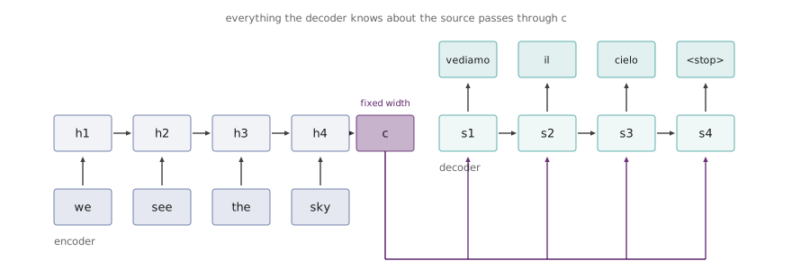
The fix suggests itself once the defect is stated that way. Do not summarize once. Let the decoder look back at the whole input sequence each time it produces a word, and build whatever summary that particular word needs. Nothing then has to survive a lossy compression, and nothing has to be decided before the decoder knows what it is about to say.

9.2 Looking back

Turning that intent into a differentiable mechanism takes three operations, applied afresh at every decoder step. Bahdanau, Cho and Bengio introduced them in 2015 and the shape has not changed since.

Start with the decoder’s current state $s_{t-1}$, which encodes what the decoder has said so far and therefore what it needs next. Compare it against each encoder state in turn to produce a scalar per input position,

$$e_{t,i} = f_{\text{att}}(s_{t-1},\, h_i) \tag{9.2}$$

where $f_{\text{att}}$ is a small learned network — concatenate the two vectors, push them through a linear layer, read off one number. The number is an alignment score: how relevant input position $i$ is to what the decoder is about to emit at step $t$. Nothing constrains it. It is a real number of arbitrary sign and magnitude, one per input position, and for a four-word source there are four of them.

Unbounded scores are awkward to combine, so the second operation is a softmax across the input positions,

$$a_{t,i} = \frac{\exp(e_{t,i})}{\sum_{j} \exp(e_{t,j})} \tag{9.3}$$

which turns the scores into a distribution: every $a_{t,i}$ lies between zero and one and the whole set sums to one. What has been computed at this point is a probability distribution over positions in the source, conditioned on where the decoder stands. Call these the attention weights.

The third operation spends them. Take the encoder states and average them under that distribution,

$$c_t = \sum_{i} a_{t,i}\, h_i \tag{9.4}$$

which gives a context vector built for step $t$ alone. If the weights concentrate on positions one and two, $c_t$ is essentially $h_1$ and $h_2$ blended; if they spread evenly, $c_t$ is the mean of everything. The decoder update is unchanged from Equation 9.1 — same three arguments, same recurrent unit — except that the constant $c$ has become $c_t$, recomputed at every step from the same encoder states through the same $f_{\text{att}}$.

Figure 9.2: One decoder step with attention. The decoder state $s_{t-1}$ is compared against every encoder state to give scores $e_{t,i}$ (Equation 9.2), a softmax turns those into weights $a_{t,i}$ that sum to one (Equation 9.3), and the encoder states are averaged under those weights to give this step’s context vector $c_t$ (Equation 9.4). The same three operations run again, with the same $f_{\text{att}}$ and different $s$, at every step of the output. Drawn for these notes.

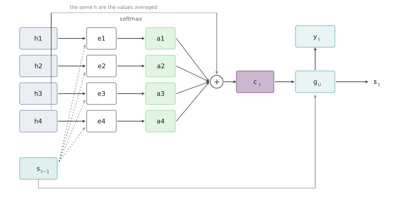
The bottleneck is gone in the literal sense: there is no longer a fixed-size channel through which everything about the source must pass, because the decoder reads the encoder states directly and reads them anew each time. A source of a thousand words presents a thousand states, and the decoder is free to draw on any of them at any step.

What makes the mechanism work is not the intuition behind it but the fact that every operation in Equation 9.2 through Equation 9.4 is differentiable. Nothing supervises the weights. There is no annotated alignment in the training data, no signal that says vediamo covers we see; the only loss is the usual cross-entropy on the output tokens, and the gradient of that loss flows back through the weighted sum, through the softmax, into $f_{\text{att}}$, and on into the encoder. The model discovers that concentrating on the right source words makes the next word easier to predict, and it discovers this because concentrating on the wrong ones costs loss. Had the alignment needed supervising, the method would have died on the training data alone.

Two details of the recurrent framing are worth keeping straight, because they are easy to conflate. The decoder’s weights are initialized the way any network’s are, at random, and learned by gradient descent. The decoder’s initial state $s_0$ is a different question, answered at the start of each sequence: sometimes the encoder’s final state, sometimes a learned projection of it, sometimes zeros. Any of the three works provided the network is trained with the one it will be given.

9.3 What the weights show

Because the weights are a distribution over source positions and there is one distribution per output step, a trained model hands over a matrix: one row per word it produced, one column per word it read, every row summing to one. That matrix is readable, and reading it is the first thing attention gave the field that was not a performance number.

Figure 9.3: The structure a learned alignment tends to have, drawn as a heat map with source words across the top and generated words down the side; brighter cells carry more weight. The mass sits near the diagonal because the two languages largely agree on order, and departs from it where they do not — the adjective and noun that swap places produce the crossing near the middle, and a phrase covered by a single word in the target draws weight from more than one column. This is a schematic of the structure, evaluated by the figure script; it is not the output of a trained model. Drawn for these notes.

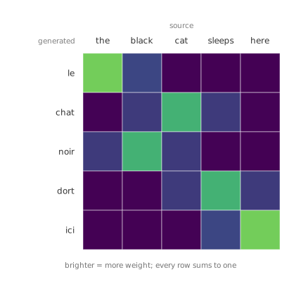
What such matrices show, for a pair of languages that mostly agree on word order, is a bright band along the diagonal that leaves it exactly where the languages disagree — adjective and noun exchanging places in French, a compound in one language covered by two words in the other. The band is soft rather than sharp. A word rarely attends to precisely one source word and nothing else; it attends mostly to one and a little to its neighbours, which is the difference between an alignment learned as a continuous quantity and one imposed as a discrete matching.

The model was never told any of this. It was told to predict the next Italian word and it inferred the correspondence as a by-product, which is worth pausing on: a mechanism introduced to widen a channel turned out to also expose what the network was using the channel for. That secondary property is why attention weights are now routinely plotted over images, over tokens and over patches whenever someone wants to ask a trained model what it was looking at — though the answer they give is where the weights went, which is not always the same as what the model relied on.

9.4 Attention as a layer in its own right

Nothing in Equation 9.2 through Equation 9.4 mentions translation, and on inspection very little of it mentions recurrence either. The mechanism takes one vector standing for a request, a set of vectors standing for available information, and returns a weighted blend of the second chosen by comparison with the first. The encoder states could be anything; the decoder state could be anything. What follows detaches the mechanism from the model it was invented inside, and the result is a layer that can be used anywhere.

Fix the vocabulary first, because the general version needs names that do not presume an encoder. The vector expressing what is wanted is the query $q$. The vectors that can be looked at are the inputs $x_1, \dots, x_N$. The comparison produces a similarity, the similarities are normalized, and the inputs are averaged. So far this is a renaming, and three generalizations turn it into something better.

The first replaces the learned comparison $f_{\text{att}}$ with a plain dot product, $e_i = q \cdot x_i$. This is a reduction in expressive power and it buys parallelism: a dot product between a query and $N$ inputs is a matrix–vector product, which hardware does at full speed, whereas $f_{\text{att}}$ is a small neural network evaluated $N$ times. The trade turned out to be overwhelmingly worth making, and it recurs in this lecture: a mechanism that is slightly weaker per unit but expressible as a matrix multiply beats a stronger one that is not.

The dot product needs one correction before it can be used, and the correction is not cosmetic. If the query and the inputs have dimension $D$ and their entries are roughly independent with unit variance, the dot product is a sum of $D$ such products and its typical magnitude grows like $\sqrt{D}$. Large-magnitude scores make the softmax of Equation 9.3 peaked: with a few hundred dimensions the largest score wins almost all of the mass, the distribution approaches a one-hot vector, and the softmax’s gradient there is nearly zero. Training then stalls, not because the model is wrong but because the scores were too large. Dividing by $\sqrt{D}$ removes the dimension’s effect on scale:

$$e_i = \frac{q \cdot x_i}{\sqrt{D}} \tag{9.5}$$

This is the scaled dot product, and the scaling is what keeps the gradient alive as models grow wide.

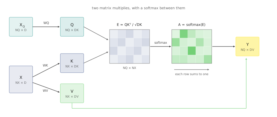
The second generalization lets several queries be answered at once. There is no reason to process one query at a time, and in every use below there are many: pack them as the rows of a matrix $Q$ of shape $N_Q \times D$ and the inputs as the rows of $X$ of shape $N_X \times D$. Then every score for every query is one matrix multiply,

$$E = \frac{Q X^{\top}}{\sqrt{D}} \tag{9.6}$$

giving an $N_Q \times N_X$ matrix whose entry $E_{i,j}$ is query $i$ against input $j$. Softmax is applied along the input axis, so that each query’s row of weights sums to one, and the weighted sums of Equation 9.4 are a second matrix multiply,

$$A = \operatorname{softmax}(E), \qquad Y = A X \tag{9.7}$$

with $Y$ of shape $N_Q \times D$: one output vector per query. Two matrix multiplies and a softmax between them, and the layer is done.

Note

Which axis the softmax runs along is the detail most often got wrong when implementing this, and getting it wrong produces a network that trains to something mediocre rather than one that fails loudly. The weights for a given query must form a distribution over the inputs, so the normalization is along the axis indexing inputs. With $E$ laid out as queries × inputs, that is the row.

9.5 Keys and values

The third generalization is the one that turns a retrieval rule into a learnable layer, and the argument for it is worth making slowly because the mechanism as stated has a conflict buried in it.

Each input vector $x_i$ is doing two jobs. It is what the query is compared against, and it is what gets returned when the comparison succeeds. Those are different jobs and there is no reason the same vector should be good at both. The features that make a word findable — its position in the sentence, its part of speech, the fact that it is the subject — need not be the features another part of the network wants to receive about it. Forcing one vector to serve both roles means every improvement to one degrades the other.

So split them. Learn two linear transformations of the inputs:

$$K = X W_K, \qquad V = X W_V \tag{9.8}$$

The keys $K$ are what queries are matched against; the values $V$ are what gets returned. The queries themselves are usually a learned projection too, $Q = X_Q W_Q$, so that the vectors doing the asking can be shaped independently of the vectors doing the answering. The layer becomes

$$Y = \operatorname{softmax}\!\left(\frac{Q K^{\top}}{\sqrt{D_K}}\right) V \tag{9.9}$$

which is the equation the rest of this chapter is about. Its parameters are three matrices, $W_Q$, $W_K$ and $W_V$, and nothing else; the attention operation itself has no weights at all.

Figure 9.4: The attention layer of Equation 9.9, with every shape marked. Queries and inputs enter on the left, the key and value projections produce $K$ and $V$, the outer product $QK^{\top}$ gives an $N_Q \times N_X$ grid of scaled scores, the softmax normalizes each query’s row into a distribution over inputs, and multiplying by $V$ returns one output vector per query. Drawn for these notes.

The database analogy is close enough to be useful and worth stating precisely so it can then be qualified. A lookup table stores key–value pairs, receives a query, finds the key that matches, and returns the corresponding value. Equation 9.9 does the same thing with two changes: the match is a graded similarity rather than an equality test, and the return is a blend of every value weighted by how well its key matched rather than a single row. Soft retrieval, in other words, and soft is what makes it differentiable — a hard lookup has no useful gradient with respect to the query, and this one does.

Notice what the layer does not assume. It takes two sets of vectors and returns one, and nothing in Equation 9.9 refers to order, adjacency, or time. It works on the words of a sentence, the patches of an image, the nodes of a graph, or an unordered pile of vectors with no structure at all. That generality is the reason the rest of the course keeps meeting this equation.

9.6 One set, attending to itself

Equation 9.9 has two inputs, $X_Q$ and $X$, and translation supplies them naturally: the decoder asks, the encoder answers. Attention used this way, with queries from one collection and keys and values from another, is cross-attention, and it is the right tool whenever a problem genuinely has two kinds of thing in it — a source sentence and a translation, an image and the caption being written about it.

Many problems have only one. Classifying an image or modelling a sentence involves a single collection of vectors that needs to be processed, with nothing external to consult. For those, take the same layer and feed it the same set three times:

$$Q = X W_Q, \qquad K = X W_K, \qquad V = X W_V \tag{9.10}$$

with all three projections applied to the same $N \times D$ matrix of inputs. This is self-attention. Every vector emits a query describing what it wants to know, a key advertising what it offers, and a value carrying what it will hand over; then every vector’s query is compared against every vector’s key and each output is the corresponding blend of values. Nothing else changes. Everything above the projections in Figure 9.4 — the scores, the softmax, the weighted sum — is unmodified, and the layer maps $N$ input vectors to $N$ output vectors, each of which has consulted all the others.

The three projections in Equation 9.10 are usually computed as one matrix multiply rather than three, by concatenating $W_Q$, $W_K$ and $W_V$ into a single $D \times 3D$ matrix. This changes nothing mathematically and matters in practice: hardware prefers a few large matrix multiplies to many small ones, and the fused projection is what implementations do.

9.6.1 The layer does not know what order the inputs came in

Shuffle the rows of $X$ and follow the consequences through Equation 9.10. The queries, keys and values are computed row by row, so they come out identical but shuffled. The scores $E_{ij} = q_i \cdot k_j / \sqrt{D_K}$ compare the same pairs of vectors as before, so the score matrix has the same entries with its rows and columns permuted the same way. Softmax normalizes each row independently and does not care what order the rows arrive in. The weighted sums pair the same weights with the same values. So the outputs are the same vectors, permuted exactly as the inputs were:

$$F(\sigma(X)) = \sigma(F(X)) \tag{9.11}$$

for any permutation $\sigma$. Self-attention is permutation equivariant, which is the same relation Section 6.11 established for convolution and translation, with a different group acting.

The consequence is worth stating bluntly, because it is easy to slide past. Self-attention does not operate on sequences. It operates on sets. The vectors happen to be packed into a matrix and a matrix has rows in an order, but the layer’s computation is blind to that order, and any apparent sensitivity to sequence in a model built from these layers has to come from somewhere else.

Sometimes that blindness is exactly right: a set of object proposals or a bag of image patches has no intrinsic order to respect. Usually it is not. “The dog bit the man” and “the man bit the dog” contain the same words, so a model whose only mixing operation is self-attention cannot distinguish them.

The fix is to put the order into the inputs, since it cannot live in the layer. Attach to each input vector a positional encoding, a vector that is a fixed function of the index, either added to the input or concatenated with it. The original transformer used sinusoids of geometrically spaced frequencies,

$$p_{t,2i} = \sin\!\left(\frac{t}{10000^{2i/D}}\right), \qquad p_{t,2i+1} = \cos\!\left(\frac{t}{10000^{2i/D}}\right) \tag{9.12}$$

where $t$ is the position and $i$ indexes the dimension pair, so that each position gets a distinct pattern and nearby positions get similar ones. A learned lookup table indexed by position works about as well and is common; more recent models mostly use rotary embeddings, which encode position by rotating queries and keys so that scores depend on relative rather than absolute position. All of them do the same job: they make two otherwise identical vectors distinguishable by where they sit.

9.6.2 Blocking some of the connections

Full self-attention lets every position see every other, and there are problems where that is wrong rather than merely wasteful. Language modelling is the clear case. If the model is trained to predict the next token at every position at once, then the output at position $t$ must not depend on the tokens at positions after $t$ — otherwise it can read the answer it is being asked to produce, and the loss goes to zero without anything being learned.

Preventing that requires no new machinery. Set the disallowed scores to $-\infty$ before the softmax:

$$E_{ij} \leftarrow -\infty \quad \text{for } j > i \tag{9.13}$$

Then $\exp(-\infty) = 0$, those weights come out exactly zero, and the output at position $i$ is a blend of the values at positions $1$ through $i$ only. This is masked self-attention, and the pattern above is the causal mask; other patterns block other things — a local window, a block-diagonal restriction to within-segment attention — by the same route.

Figure 9.5: Masked self-attention. Scores above the diagonal are overwritten with $-\infty$ before the softmax, so their weights come out zero and each position blends only the values at or before it. Trained this way on “attention is very cool”, the position holding attention predicts is without ever having seen it. Drawn for these notes.

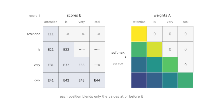
Masking is what lets self-attention take over the language-modelling job of Section 8.6 outright. The recurrent model enforced causality by construction — a state moving forward in time cannot consult the future — and paid for it with a sequential update. The masked attention layer enforces causality by arithmetic and computes every position at once.

9.7 Several heads

A single self-attention layer produces one set of weights per position, which means every position gets one distribution over what to look at. That is a real restriction. A word may need its syntactic governor, its coreferent, and the topic of the paragraph simultaneously, and one distribution cannot concentrate on three unrelated things without diluting all of them.

Run several attention layers side by side instead. Split the model dimension into $H$ heads, give each its own $W_Q$, $W_K$ and $W_V$ projecting into a head dimension $D_H$, run Equation 9.9 independently in each, concatenate the $H$ outputs back to width $H D_H$, and mix them with one more learned matrix $W_O$:

$$O = \operatorname{concat}(Y_1, \dots, Y_H)\, W_O \tag{9.14}$$

Conventionally $D_H = D / H$, so the concatenation returns to the input width and the layer is a map from $N \times D$ to $N \times D$ regardless of how many heads it has. A model with $D = 512$ and $H = 8$ gives each head 64 dimensions to work in.

Note what that convention buys: at $D_H = D/H$ the parameter count and the arithmetic are essentially independent of $H$, since the heads split the width rather than duplicating it. Eight heads of width 64 cost what one head of width 512 costs. What changes is that eight separate distributions are computed instead of one, and the heads are identical in architecture and differ only in weights — they are initialized differently and specialize because the loss rewards their specializing, not because anyone assigned them roles.

The implementation runs all heads in one batched matrix multiply rather than in a loop, which is why the whole multi-head layer, for all its indices, reduces to four matrix multiplies: the fused $QKV$ projection, the batched $QK^{\top}$, the batched weighting of $V$, and the output projection $W_O$. Multi-head is the form in which self-attention is essentially always used.

9.8 What it costs

Those four matrix multiplies are worth pricing, because two of them scale differently from the others and the difference decides what the layer can be used for.

The projections at either end — step one and step four — are applied to each vector independently, so they cost $O(N D^2)$ for $N$ vectors of width $D$: linear in the number of vectors. The two in the middle are not. Computing $QK^{\top}$ compares every query against every key, which is $N^2$ scores per head, and weighting $V$ by those scores costs the same again. Attention is $O(N^2 D)$, quadratic in the number of inputs, and no rearrangement of the algebra changes that, because the layer’s defining property is that every output consults every input.

The memory is the sharper constraint, because a naïve implementation materializes the score matrix. That is $H$ matrices of $N \times N$ held at once, and the numbers get out of hand quickly: at $N = 100{,}000$ tokens with $H = 64$ heads, the attention weights alone are $6.4 \times 10^{11}$ entries, which even at two bytes each is 1.28 terabytes. No accelerator has that. Long-context attention was for several years limited not by arithmetic but by the refusal of that matrix to fit.

FlashAttention removed the constraint by never forming the matrix. It fuses the two middle multiplies, walking over the inputs in tiles small enough to sit in on-chip memory, accumulating each output as it goes with an online softmax that never needs a whole row at once. The result is exact — this is not an approximation of attention — and the memory drops from $O(N^2)$ to $O(N)$ while the arithmetic stays quadratic. Nearly every long-context model in use depends on it.

The quadratic compute that remains is usually presented as attention’s flaw, and the presentation deserves an objection. In ordinary algorithm design a quadratic term is a defect to be engineered away. Here the term buys something: more compute spent on a sequence is more computation performed on it, and a model that does more work per input has more opportunity to arrive at a good answer. Attention’s cost is not overhead attached to the useful work; within limits it is the useful work. Expensive and useless would be a defect. Expensive and proportionately more capable is a price.

9.9 Three ways to process a sequence

The course has now built three mechanisms that turn a collection of inputs into a collection of outputs, and they are worth putting side by side, because the transformer’s design is a bet about which of the three properties matters.

Figure 9.6: The three primitives compared on how information travels between distant positions. The recurrent network passes it along a chain, so distance costs sequential steps. The convolution mixes locally, so distance costs depth. Self-attention connects every position to every other in one layer, so distance costs nothing — and every connection is drawn, which is also the picture of why it costs $O(N^2)$. Drawn for these notes.

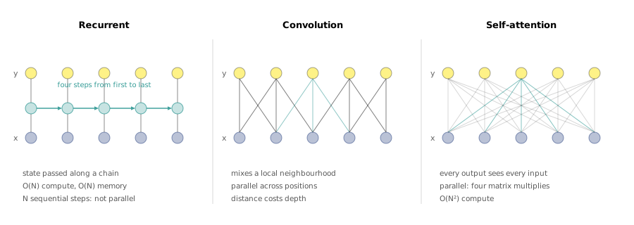
A recurrent network works on one-dimensional ordered sequences and processes them in $O(N)$ compute and memory, which is the best of the three. Its defect is that the recurrence is inherently serial: $h_t$ cannot be computed before $h_{t-1}$, so a sequence of length $N$ takes $N$ sequential steps no matter how much hardware is available.

A convolution works on grids of any dimension and is embarrassingly parallel — every output position is independent of every other. Its defect is reach. A single layer mixes information only within its kernel, so relating two distant positions requires either enormous kernels or a deep stack, and Section 6.8 showed exactly how slowly the receptive field grows.

Self-attention works on sets, with no assumption of order or grid. Every output depends directly on every input after one layer, so distance costs nothing, and the whole operation is four matrix multiplies, which parallelize as well as anything in computing. Its defect is the quadratic cost just described.

The reason the third property is decisive is a fact about hardware rather than about sequences. Single processors stopped getting appreciably faster some time ago; what has continued to grow, by orders of magnitude, is how many processors can be pointed at one problem. An algorithm that can only use one fast processor is stuck waiting on a trend that has ended, while an algorithm that can spread over a thousand of them rides the one that has not. Recurrence is the first kind and attention is the second, and that — more than any argument about which mechanism is a better model of language — is why the field went the way it did.

9.10 The transformer block

Vaswani et al. put self-attention at the centre of an architecture in 2017 and used the title to say how far they were prepared to take the idea. The block they defined is short enough to state completely and has barely changed since.

Take a set of vectors $x$. Pass them through multi-head self-attention, which is the only operation in the whole block where vectors see each other. Wrap it in a residual connection, for the reasons Section 7.8 gave: a path that skips the transformation keeps the gradient intact through a deep stack. Normalize, with layer normalization — the variant of Section 7.2 that standardizes each vector across its own features, using no statistics from other vectors and therefore none from other positions, which is what makes it safe here.

Then do something quite different. Self-attention mixes information between vectors and computes nothing much within one; the weighted sum of values is a linear operation, and stacking such layers would compose into another linear map on the set. So the block adds a second primitive: a small MLP, applied independently and identically to each vector, conventionally two layers widening from $D$ to $4D$ and back with a nonlinearity between. It is also wrapped in a residual connection and followed by a second normalization.

$$\begin{aligned} z &= \operatorname{LayerNorm}\big(x + \operatorname{MultiHeadAttn}(x)\big) \\ y &= \operatorname{LayerNorm}\big(z + \operatorname{MLP}(z)\big) \end{aligned} \tag{9.15}$$

Figure 9.7: The transformer block of Equation 9.15. Self-attention is the only operation in which vectors interact; layer normalization and the MLP act on each vector alone. Both sublayers sit inside residual connections. A transformer is this block repeated, with new weights each time and no change of shape. Drawn for these notes.

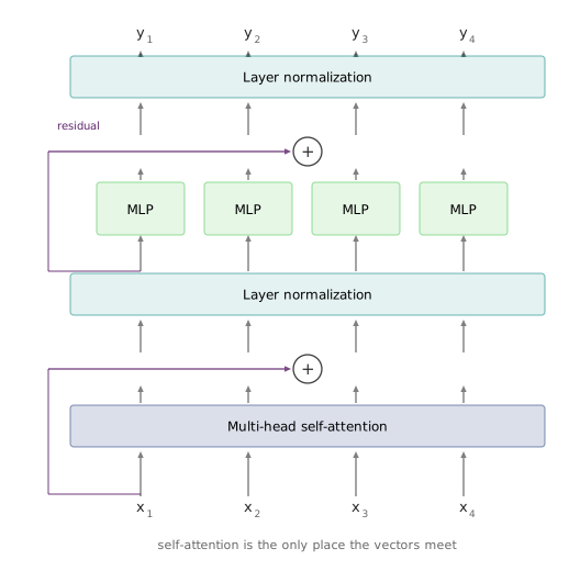
The division of labour is the design. Every position gets a chance to gather what it needs from everywhere else, then a chance to think about what it gathered, alternating for as many blocks as the model has. Because the block maps $N \times D$ to $N \times D$, blocks compose without any bookkeeping: a transformer is a stack of them, identical in shape, each with its own weights. Six matrix multiplies dominate the cost — four from attention, two from the MLP — and every one of them is large and batched, which is the property Section 9.9 argued was decisive.

What has changed since 2017 is scale, not structure. The original model in its larger configuration stacked twelve blocks at $D = 1024$ with sixteen heads, 213 million parameters in all. GPT-2 two years later ran 48 blocks at $D = 1600$ with 25 heads for 1.5 billion parameters, and GPT-3 the year after that ran 96 blocks at $D = 12288$ with 96 heads for 175 billion. Across three orders of magnitude in parameters, Equation 9.15 is what was being stacked.

9.11 Stacking blocks into a language model

The blocks handle vectors, and words are not vectors, so a language model needs a layer at each end.

At the input, a learned embedding matrix of shape $V \times D$ for a vocabulary of size $V$: one row per token, and turning a token into a vector is a lookup. At the output, a projection of shape $D \times V$ turning each block’s output vector back into a score per vocabulary entry, which a softmax and a cross-entropy loss compare against the token that actually came next. In between, blocks whose attention is masked as in Equation 9.13, so position $t$ sees only positions up to $t$.

That is the entire architecture, and the training objective is the one Section 8.6 already introduced for recurrent networks: predict the next token, with the text as its own supervision. What changes is that every position’s prediction is computed in parallel in one pass, and that the path from any token to any earlier token is one attention step rather than a chain of state updates.

9.12 The same block, on images

Nothing in Equation 9.15 mentions language. It consumes a set of vectors, so applying it to images is a question of how to turn an image into a set of vectors — and Dosovitskiy et al. answered it about as directly as possible.

Cut the image into a grid of non-overlapping square patches, typically $16 \times 16$ pixels. A $224 \times 224$ image gives $14 \times 14 = 196$ of them. Flatten each patch into a vector of $16 \cdot 16 \cdot 3 = 768$ numbers and apply one learned linear map to width $D$. Add a positional encoding, since Equation 9.11 means the block would otherwise not know where any patch sat. Feed the 196 vectors to a stack of transformer blocks — unmasked, since there is nothing to predict in sequence and every patch may see every other. Average the outputs and apply a linear layer to get class scores.

Figure 9.8: The Vision Transformer. The image is cut into fixed patches, each flattened and linearly projected to width $D$; positional encodings supply the geometry the transformer cannot infer; the blocks are the same ones Figure 9.7 draws, unmasked; and the outputs are pooled and classified. The patch projection is exactly a $16 \times 16$ convolution with stride 16, so the only convolution in the model is the one that builds its input. Drawn for these notes.

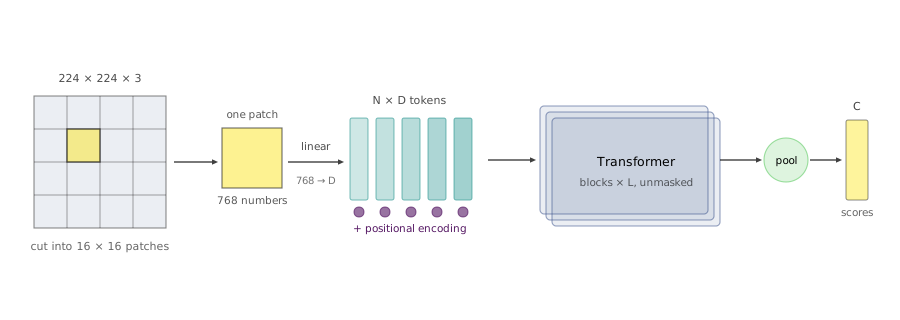
The patch step deserves a second look, because it is a familiar operation in unfamiliar dress. Cutting an image into $16 \times 16$ tiles and applying the same linear map to each is a convolution with a $16 \times 16$ kernel, stride 16, three input channels and $D$ output channels. The architecture that was presented as an alternative to convolutional networks begins with a convolution, and then contains no others — which locates the actual disagreement precisely. It is not about whether local linear filtering is useful at the very first step. It is about whether everything above that step should also be local.

9.13 What changed after 2017

Equation 9.15 is still recognisably what current models run, but four modifications have become close to standard, and a reader meeting a modern implementation will see all four. The lecture ran out of time before reaching them and left them as reading; they are short.

Pre-norm. In Equation 9.15 the normalization sits outside the residual addition, which has an awkward consequence: there is no setting of the weights for which the block computes the identity, since everything passing through is normalized on the way out. Moving each normalization to the front of its sublayer, inside the residual, restores it —

$$z = x + \operatorname{MultiHeadAttn}\big(\operatorname{Norm}(x)\big) \tag{9.16}$$

— and leaves a clean path from input to output. Deep stacks train more stably this way, without the learning-rate warmup the original arrangement needed, and it is now the default.

RMSNorm. Layer normalization subtracts each vector’s mean and divides by its standard deviation. RMSNorm drops the centering and divides by the root mean square alone,

$$y_i = \frac{x_i}{\sqrt{\varepsilon + \frac{1}{D}\sum_j x_j^2}} \, \gamma_i \tag{9.17}$$

which is cheaper, loses nothing measurable, and is what most recent models use.

SwiGLU. The classic MLP computes $\sigma(XW_1)W_2$ with a widening of $4D$. The gated variant computes two projections and lets one gate the other elementwise,

$$Y = \big(\sigma(XW_1) \odot XW_2\big)W_3 \tag{9.18}$$

with the hidden width set to $\tfrac{8}{3}D$ so that three matrices cost what two did. It works better, and the paper that introduced it declined to explain why, attributing the result “as all else, to divine benevolence.”

Mixture of experts. Learn $E$ separate MLPs per block instead of one, and route each token to $A < E$ of them, chosen by a small learned gate. Parameters scale with $E$ while the compute per token scales with $A$, which decouples how much a model knows from how much it spends per token — the reason the idea is now behind essentially every frontier model, though those models publish few enough details that this is inference rather than fact.

9.14 What this leaves

The chapter started with a single vector too narrow to carry a sentence, and every step after that was a removal. Removing the bottleneck gave a decoder that rebuilt its context at each step. Removing the decoder gave a layer taking queries against inputs. Removing the learned comparison gave a scaled dot product and with it the ability to run everything as a matrix multiply. Removing the distinction between the two input sets gave self-attention, which needed positional encodings put back precisely because the removals had gone as far as discarding order itself.

What is left is an operation on sets of vectors, parameterized by three projections, in which every element consults every other in one step. It carries no assumption about grids, adjacency, or time, which is why the same layer serves words, patches, and — in later chapters — point clouds, video frames, and pairs of modalities that have nothing structural in common. The transformer is the small amount of scaffolding needed to use that operation repeatedly: mix across positions, compute within each, wrap both in residual connections, stack.

Two things are worth carrying forward past the architecture. The first is the trade that keeps recurring: a mechanism that is weaker per unit of computation but expressible as a large matrix multiply beats a stronger one that is not, because hardware scales in width and not in speed. The second is that attention’s cost is quadratic and that this has been survivable — better arithmetic on the same operation, as in FlashAttention, has bought more than any of the many attempts to replace it with something cheaper.

The next chapter turns from architectures to tasks: detection, segmentation, and the question of what a trained network has actually learned to look at.

References

• J. L. Ba, J. R. Kiros and G. E. Hinton, “Layer Normalization,” 2016. arXiv:1607.06450
• A. Baevski and M. Auli, “Adaptive Input Representations for Neural Language Modeling,” ICLR, 2019. arXiv:1809.10853
• D. Bahdanau, K. Cho and Y. Bengio, “Neural Machine Translation by Jointly Learning to Align and Translate,” ICLR, 2015. arXiv:1409.0473
• T. Brown et al., “Language Models Are Few-Shot Learners,” NeurIPS, 2020. arXiv:2005.14165
• T. Dao, D. Y. Fu, S. Ermon, A. Rudra and C. Ré, “FlashAttention: Fast and Memory-Efficient Exact Attention with IO-Awareness,” NeurIPS, 2022. arXiv:2205.14135
• A. Dosovitskiy et al., “An Image Is Worth 16x16 Words: Transformers for Image Recognition at Scale,” ICLR, 2021. arXiv:2010.11929
• M.-T. Luong, H. Pham and C. D. Manning, “Effective Approaches to Attention-Based Neural Machine Translation,” EMNLP, 2015. arXiv:1508.04025
• N. Shazeer, “GLU Variants Improve Transformer,” 2020. arXiv:2002.05202
• N. Shazeer et al., “Outrageously Large Neural Networks: The Sparsely-Gated Mixture-of-Experts Layer,” ICLR, 2017. arXiv:1701.06538
• J. Su et al., “RoFormer: Enhanced Transformer with Rotary Position Embedding,” 2021. arXiv:2104.09864
• I. Sutskever, O. Vinyals and Q. V. Le, “Sequence to Sequence Learning with Neural Networks,” NeurIPS, 2014. arXiv:1409.3215
• A. Vaswani et al., “Attention Is All You Need,” NeurIPS, 2017. arXiv:1706.03762
• B. Zhang and R. Sennrich, “Root Mean Square Layer Normalization,” NeurIPS, 2019. arXiv:1910.07467