17  Vision and Language

Lecture 16

Based on Lecture 16 of CS231n, Stanford University, Spring 2025, given by Ranjay Krishna.

17.1 One model, or one model per task

Every chapter so far has described the same loop, and described it so consistently that the loop stopped looking like a choice. Collect a dataset with a training split and a test split. Train a model on the training split for the one task the dataset was built to measure. Report a number on the test split. Detection, segmentation, captioning, video classification — each got its own dataset, its own architecture, its own training run, and its own leaderboard, and a model that was excellent at one of them was, in the strict sense, useless at any other. The weights encoded a task as much as they encoded the world.

What changed is not that anyone found a better architecture for image classification. What changed is the observation, arriving from language first, that the expensive part of training is learning what things are, and the cheap part is learning what to do with them. If the expensive part can be paid once, on data that is not organised around any particular task, then the cheap part can be paid many times over, in some cases with a handful of examples and in some cases with none at all. A model trained that way is called a foundation model, and the name is doing real work: it is a claim about position in a pipeline rather than about architecture.

The definition is contested at the edges, and the lecture is honest about this. The one property everyone agrees on is generality — the same weights serve many downstream tasks without being retrained for each. The properties that usually accompany it but do not define it are the familiar three: a large parameter count, a large and diverse pretraining corpus, and a self-supervised objective. Those three are means rather than ends. A model can have all of them and remain a specialist, and the interesting question about any candidate foundation model is not how large it is but how little you have to do to it before it is useful for something its authors did not anticipate.

Language got there first, and got there for a reason worth stating plainly, because it is the constraint that everything in this chapter is working around. Text is self-labelling. The next word in a sentence is both the input to the model and the supervision for it, and there is no annotation step between a web crawl and a training corpus. That single property is what let language models scale to corpora nobody could have labelled, and it is exactly what vision lacked. Pixels do not come with their next pixel in any semantically useful sense, and the self-supervised objectives of Section 13.9 — asking two augmentations of one image to agree — produce representations without producing an interface. A SimCLR encoder maps a photograph to a good vector. Nothing about that vector tells you what the photograph is of, and recovering that still needs a labelled dataset and a supervised head.

So the vision story of the last five years is best read as a search for something that plays the role that next-word prediction plays in language: a supervision signal that already exists at web scale, that nobody has to pay for, and that carries semantics rather than just invariance. The answer turned out to be text — not as the output of the vision model but as its supervisor.

17.2 Text as the label that already exists

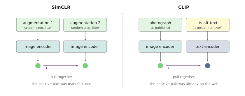
Recall the shape of the SimCLR objective. Take an image, produce two augmentations of it, push their representations together, and push them away from the representations of every other image in the batch. The positive pair is manufactured — it exists because the augmentation pipeline made it — and the negatives are whatever else happened to be in the minibatch. The model learns to be invariant to crops, colour jitter and blur, which is a real and useful thing to learn, but the semantics come in only by implication: two crops of a cat share a label because they share an origin, not because anything in the loss knows the word cat.

CLIP changes exactly one thing about that picture, and the change is small enough to state in a sentence and consequential enough to have reorganised the field. Keep the image encoder on the left. Replace the second image encoder on the right with a text encoder. The positive pair is no longer two augmentations of one photograph; it is a photograph and the caption that was published alongside it. Everything else — the contrastive form, the in-batch negatives, the temperature — carries over unchanged.

Figure 17.1: The move from SimCLR to CLIP. Both objectives pull a positive pair together and push everything else in the batch apart; they differ only in where the positive pair comes from. SimCLR manufactures it with augmentation, so the model learns invariance. CLIP takes it from the web, so the model learns to associate an image with a description — and inherits an interface it can be queried through.

Write the batch as $N$ pairs $(x_i, y_i)$ of image and caption, and let $u_i = g_{\text{img}}(x_i)$ and $v_i = g_{\text{txt}}(y_i)$ be the two encoders’ outputs after projection to a shared space and normalisation to unit length, so that $\langle u_i, v_j \rangle$ is a cosine similarity in $[-1, 1]$. The batch defines an $N \times N$ matrix of these similarities, and the entire training signal is the claim that its diagonal should dominate. Reading the matrix along its rows gives the image-to-text loss,

$$\mathcal{L}_{\text{I}\to\text{T}} = -\frac{1}{N}\sum_{i=1}^{N} \log \frac{\exp\!\left(\langle u_i, v_i \rangle / \tau\right)} {\sum_{j=1}^{N} \exp\!\left(\langle u_i, v_j \rangle / \tau\right)}, \tag{17.1}$$

which asks each image to select its own caption out of the $N$ on offer. Here $\tau$ is a learned temperature that sets how sharply the softmax discriminates: small $\tau$ makes the loss care intensely about the single closest competitor, large $\tau$ spreads the pressure across all of them. Reading the same matrix along its columns gives the complementary constraint, that each caption should select its own image,

$$\mathcal{L}_{\text{T}\to\text{I}} = -\frac{1}{N}\sum_{j=1}^{N} \log \frac{\exp\!\left(\langle u_j, v_j \rangle / \tau\right)} {\sum_{i=1}^{N} \exp\!\left(\langle u_i, v_j \rangle / \tau\right)}, \tag{17.2}$$

and the objective actually optimised is the average of the two. The symmetry is not decoration. A one-sided loss can be driven down by an encoder that spreads images out and collapses text, or the reverse; requiring both directions to work forces both spaces to be informative.

Figure 17.2: CLIP’s training step in full. A batch of $N$ image–caption pairs produces an $N \times N$ matrix of cosine similarities; the $N$ diagonal entries are the positives and every off-diagonal entry is a negative. Cross-entropy along the rows is Equation 17.1, along the columns Equation 17.2, and the loss is their average. Every negative is free — it is another example’s positive, reused.

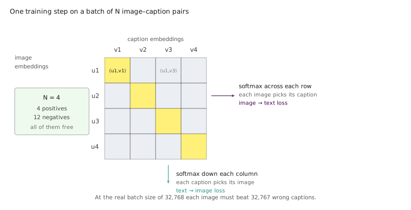
Two things about Figure 17.2 are worth dwelling on, because they explain why this objective and not a more obvious one. The first is that the negatives cost nothing. A batch of $N$ pairs yields $N$ positives and $N^2 - N$ negatives, all of them assembled by matrix multiplication from encodings that had to be computed anyway. This is why batch size is a first-class hyperparameter rather than a memory-management detail: CLIP trains at a minibatch of 32,768, and the difficulty of the discrimination problem — how many wrong captions each image has to beat — grows with it. The second is that the loss never asks either encoder to reconstruct anything. It only asks them to agree on an ordering. That is a far weaker requirement than generation, it is what makes the objective cheap, and in Section 17.5 it turns out to be exactly what the model exploits.

The payoff is the data. Alt-text is attached to images across the web for reasons that have nothing to do with machine learning, and it was already there. CLIP’s corpus is 400 million image–text pairs collected from public sources, and no one annotated any of it. This is the property that self-supervised vision objectives were reaching for and could not get: not merely unlabelled data, but data whose labels are semantic and free. The augmentation-based objectives could scale, but everything they scaled was invariance. Adding text to the same machinery scales meaning.

17.3 A similarity model is already a classifier

What comes out of training is not a classifier. It is a function that scores how well an image and a piece of text go together, which is an odd artefact if what you wanted was ImageNet accuracy. The move that turns one into the other is simple enough to feel like a trick and is, in a way that matters, not a trick at all.

Suppose you want to classify images into $C$ categories. Write each category name into a short phrase — a photo of a {label} — and push all $C$ phrases through the text encoder. That gives $C$ unit vectors $v_1, \dots, v_C$, one per class, computed once and cached. To classify a new image, encode it to $u$ and take the class whose vector it is closest to:

$$\hat{y}(x) = \arg\max_{c \in \{1, \dots, C\}} \; \langle u(x),\, v_c \rangle . \tag{17.3}$$

The lecture describes this as nearest-neighbour classification with one exemplar per class, where the exemplars happen to have been written rather than photographed, and that is a good way to hold it. But it is worth noticing what Equation 17.3 is in more familiar terms. Stack the $v_c$ as the rows of a matrix $W \in \mathbb{R}^{C \times d}$; then $\langle u, v_c \rangle$ is the $c$-th component of $Wu$, and the prediction is $\arg\max_c (Wu)_c$. This is exactly a linear classification head with no bias term, of the kind every chapter since Section 3.4 has been training with labelled data and gradient descent. CLIP does not avoid the linear head. It synthesises the weights from language instead of fitting them to examples, and the figure below makes the equivalence explicit because it is the cleanest statement of what zero-shot transfer actually is.

Figure 17.3: Constructing a zero-shot classifier. The class names are written into prompts, encoded once, and cached; classifying an image is a single matrix–vector product against them. The right-hand panel is the same computation drawn as the bias-free linear layer it is — the weights were written rather than trained, and the classifier can be rebuilt for a new label set in the time it takes to encode $C$ short strings.

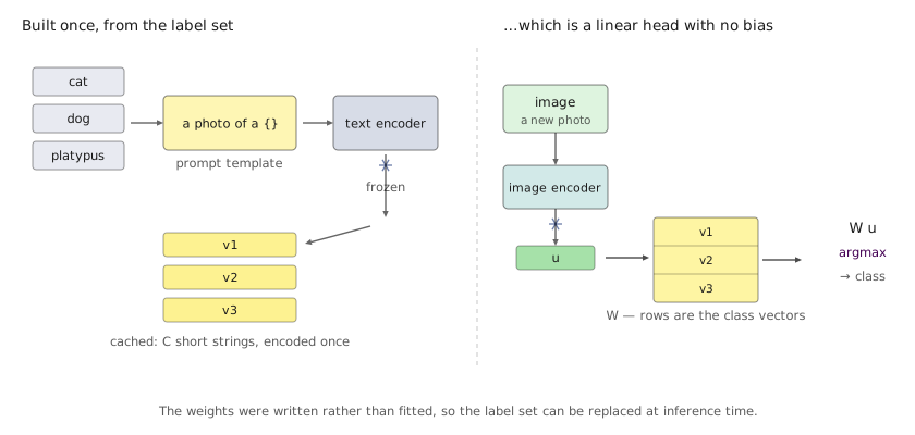
Reading it that way also explains the property that makes it useful. A trained linear head is welded to the label set it was fitted on; changing the classes means collecting examples and refitting. A written head can be rebuilt for any label set at all, including categories that appeared nowhere in training and including label sets invented at inference time. The vocabulary of the classifier is open, and its cost is a forward pass over a few short strings.

The phrasing of those strings turns out to matter more than it should, and the reasons are instructive. The text encoder was trained on captions, which are sentences, so feeding it a bare token like boxer puts it well outside the distribution it learned on — and lands it on a genuine ambiguity, since the word is a dog breed and an athlete and CLIP has seen both. Wrapping the label in a photo of a {label} recovers the caption-like form and disambiguates by context, and adding a domain hint — a satellite photo of a {label}, a sketch of a {label} — helps further on datasets where the images are not ordinary photographs.

Any single template also bakes in a bias, and the fix generalises the trick rather than tuning it. Encode the class through many templates and average the resulting vectors, renormalising the result to unit length:

$$\bar{v}_c = \frac{\frac{1}{K}\sum_{k=1}^{K} t\!\left(\text{prompt}_k(c)\right)} {\left\lVert \frac{1}{K}\sum_{k=1}^{K} t\!\left(\text{prompt}_k(c)\right) \right\rVert} . \tag{17.4}$$

CLIP ensembles 80 context prompts on ImageNet this way, worth 3.5 percentage points over the single default template, with prompt engineering and ensembling together contributing almost five points. The detail that makes it practical is where the averaging happens. Ensembling in probability space would mean running $K$ classifiers per image and averaging their outputs, so inference cost would scale with $K$. Averaging in embedding space collapses the $K$ templates into one cached vector per class before any image arrives, so the ensemble costs $K$ text encodings once and nothing at all per image thereafter. The two are not the same computation and do not give the same answer — Equation 17.4 commits to a single direction per class rather than to a mixture — but the one that is free is also the one that works.

17.4 What the zero-shot number was hiding

Trained on 400 million pairs, CLIP reaches 76.2% zero-shot top-1 on ImageNet, matching the original ResNet-50 while using none of ImageNet’s 1.28 million labelled training images. That is a striking sentence and, taken alone, a slightly boring result: a great deal of machinery to arrive where supervised training arrived years earlier. The interesting part is what happens when a supervised model matched to the same 76.2% — the paper’s comparison uses a ResNet-101 — is asked about anything else.

The benchmark suite for this measures distribution shift: datasets built from the same thousand ImageNet categories, rendered in ways the original photographs were not. ImageNetV2 is a fresh collection following the original protocol, ImageNet Sketch replaces photographs with line drawings, ImageNet-R with artistic renditions, ObjectNet photographs household objects at unusual angles and in unusual settings, and ImageNet-A collects natural photographs that standard classifiers get wrong. Nothing in any of them requires a concept the model has not been asked about. Only the pixel statistics move.

Figure 17.4: Two models matched exactly on ImageNet and separated by up to 74 points everywhere else. Bars are top-1 accuracy for a supervised ResNet-101 and for zero-shot CLIP on the six evaluations; the annotation on each pair is the gap. The supervised model’s accuracy tracks how closely a dataset resembles ImageNet’s photographs, which is the definition of having learned the dataset rather than the categories.

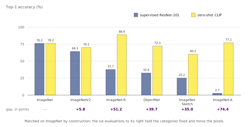
The gaps in Figure 17.4 are not the usual few points of benchmark noise. On ImageNet-R the supervised model scores 37.7% and CLIP 88.9%. On ObjectNet, 32.6% against 72.3%. On ImageNet-A, 2.7% against 77.1% — a supervised classifier performing several times worse than random guessing among a thousand classes would, because the images were selected adversarially against exactly that kind of model. The supervised network’s accuracy degrades in near-perfect proportion to how far a dataset drifts from ImageNet’s particular photographic conventions, which is the operational definition of having fitted the dataset rather than the categories. Its 76.2% was never a measurement of whether it knows what a teapot is; it was a measurement of whether it knows what an ImageNet teapot looks like. CLIP, having never seen ImageNet’s training distribution, has nothing of that kind to overfit.

This is the result that ended the argument, and it did so by reframing what the argument was about. The case for supervised pretraining had always been that labels are the most informative signal available per example, which is true. The case against is that a fixed label set caps what can be learned per example at $\log_2 1000 \approx 10$ bits, and worse, that it teaches the model the photographer’s conventions along with the category. Captions are noisier per example and unbounded in what they can express, and there are three orders of magnitude more of them.

The scaling evidence points the same way. CLIP’s zero-shot ImageNet accuracy rises steadily with both model size and data volume across the range they trained, with no sign of the saturation that supervised ImageNet training hits once the labels are exhausted — the ceiling in the supervised case is a property of the dataset, not of the method.

CoCa then showed that the contrastive objective, for all its efficiency, is leaving something on the table. Its architecture keeps CLIP’s two towers and splits the text side in two: the first block of decoder layers has no cross-attention and produces a unimodal text embedding, which is contrasted against the image embedding exactly as before, and the remaining layers cross-attend to the image features and are trained to generate the caption. One forward pass, two losses. The captioning term is a strictly harder requirement — predicting each word given the image and the preceding words demands that the image features retain the information a description needs, not merely enough to be ranked above the other images in a batch. CoCa reaches 86.3% zero-shot top-1 on ImageNet, 90.6% with a frozen encoder and a learned head, and 91.0% after fine-tuning. Contrastive pretraining is cheap and generative pretraining is informative, and the two compose.

17.5 The failure the objective permits

It would be easy to read the previous section as a straightforward win, and the lecture is careful not to let it stand that way. CLIP-style models are cheap to train relative to what they can do, trivial to retarget at a new label set, and robust in a way that supervised classifiers are not. They are also, in a specific and well-documented sense, not doing what their zero-shot numbers suggest.

Start from what Equation 17.1 actually demands. To drive the loss down, the image encoding of a photograph must score higher against its own caption than against the $N-1$ other captions in that batch — and those captions are drawn at random from the web. A batch containing a golden retriever, a plate of sushi and a suspension bridge poses a problem that is completely solved by detecting which nouns are present. Nothing about word order, nothing about which adjective attaches to which noun, and nothing about the relation between two objects is ever load-bearing, because no random negative ever differs from the positive on those axes alone. The gradient has no reason to encode structure it is never tested on, and it does not.

Figure 17.5: Why random negatives never force compositional structure. Against the batch on the left, matching nouns is a complete solution and every gradient step rewards it. The hard negatives on the right — same words, different structure — are the ones that would require more, and the probability of drawing one from a web-scale corpus at random is effectively zero.

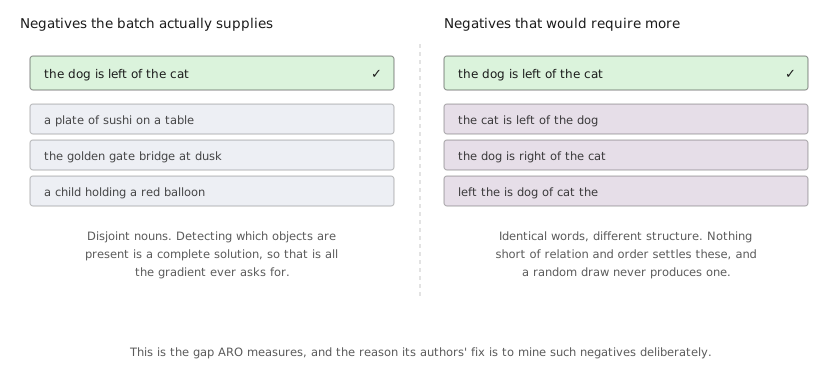
The ARO benchmark makes this precise by constructing the negatives the training distribution never supplies. Its cases are built from Visual Genome and COCO by perturbing a true caption in exactly one structural way — swapping the arguments of a relation, reassigning an attribute to the wrong object, or shuffling word order — so that the correct and incorrect captions contain the same words and differ only in how those words compose. Across more than fifty thousand such cases, state-of-the-art vision–language models behave like bags of words: relational understanding is poor, attribute-to-object binding blunders, and order sensitivity is close to absent. The authors’ diagnosis is the same as the one above, and their fix follows from it — mine hard negatives that differ compositionally, so that the objective finally has to represent what it was never asked about.

The related Winoground probe is smaller and sharper: two images and two captions built from identical words in different orders, where the task is to match them correctly. Models that score respectably on ImageNet perform at or below chance on it.

The other limitation is structural rather than statistical, and it constrains everything the rest of the chapter builds. CLIP emits one vector per image. Whatever grounding the model has — which pixels correspond to which word — is destroyed by the pooling that produces that vector, and there is no output head through which it could be recovered. The model can tell you a photograph is consistent with two dogs on a sofa. It cannot tell you where either dog is, and it is unreliable about whether there are two, because counting requires exactly the compositional structure the objective declined to learn. A single similarity score is a narrow interface, and the next three sections are each a different answer to the question of what to attach to a vision encoder so that something richer can come out.

17.6 Fusion by concatenation

If a single vector is too narrow an interface, the obvious thing to want is a model that takes an image and a question and answers in free text. By 2023 one half of that was solved — instruction-tuned language models could hold a conversation, follow directions, and reason in text — and the other half, a vision encoder producing semantically rich features, had been solved by CLIP. The question was how to join them, and there are two good answers. LLaVA takes the simpler one.

Recall that a transformer language model does not consume words. It consumes a sequence of vectors in $\mathbb{R}^{d}$, produced by looking each token up in an embedding table, and self-attention is indifferent to where in the sequence any particular vector came from. That indifference is the opening. If image content can be written as a handful of vectors in that same $d$-dimensional space, it can be concatenated into the prompt and the language model will attend to it exactly as it attends to words — with no architectural change whatsoever.

LLaVA does precisely that. A frozen CLIP ViT-L/14 encodes the image into patch features $Z$; a single trainable projection $W$ maps each patch feature into the language model’s embedding dimension, giving visual tokens $H_v = W Z$; those tokens are prepended to the embedded text tokens; and the whole sequence goes into Vicuna, which generates the response autoregressively. The connector is one matrix.

Figure 17.6: LLaVA’s fusion. Patch features from a frozen CLIP encoder are mapped by a single linear projection into the language model’s embedding space and concatenated with the text tokens, so self-attention mixes the two modalities with no change to the language model’s architecture. The connector is the only new parameter block in stage one.

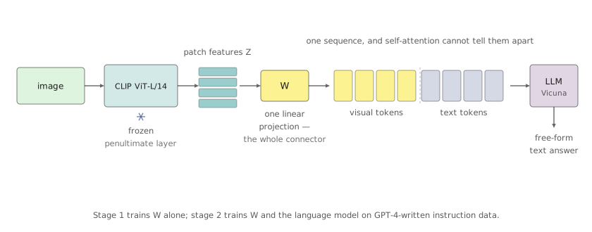
Two choices inside that simplicity carry weight. The first is which layer of the vision encoder to read. The final layer of a CLIP image encoder is trained to produce the single pooled vector that enters Equation 17.1, which means it has been optimised to discard everything not needed for that ranking — precisely the spatial detail a question-answering model wants. The penultimate layer’s patch features have not yet been through that bottleneck, and LLaVA uses them. It is the same instinct as taking features from before the classifier in transfer learning, applied to a bottleneck that is contrastive rather than categorical.

The second is where the training data comes from, and it is the part that generalised. There was no corpus of multimodal instruction-following conversations, and collecting one by hand is expensive. So LLaVA manufactured it: take images from COCO with their existing captions and bounding boxes, feed those text annotations — not the images — to a language-only GPT-4, and ask it to write conversations, detailed descriptions, and reasoning questions about the scene it can infer from them. The teacher never sees a pixel; the symbolic annotations stand in for the image, and the student learns to produce the same responses from the image itself. Training then runs in two stages, first aligning the projection with the language model frozen, then fine-tuning the projection and the language model together on the generated instruction data. The result reaches 85.1% of GPT-4’s score on a synthetic multimodal instruction benchmark and, ensembled with GPT-4, 92.53% on ScienceQA.

The honest caveat is that this is distillation. The ceiling of a model trained this way is set by the teacher that wrote its training data, which is the specific problem Section 17.8 exists to solve.

17.7 Fusion by cross-attention

Flamingo answers the same question differently, and the differences are motivated by a goal LLaVA does not pursue: keeping the language model exactly intact while teaching it to see, so that its in-context learning ability survives the operation.

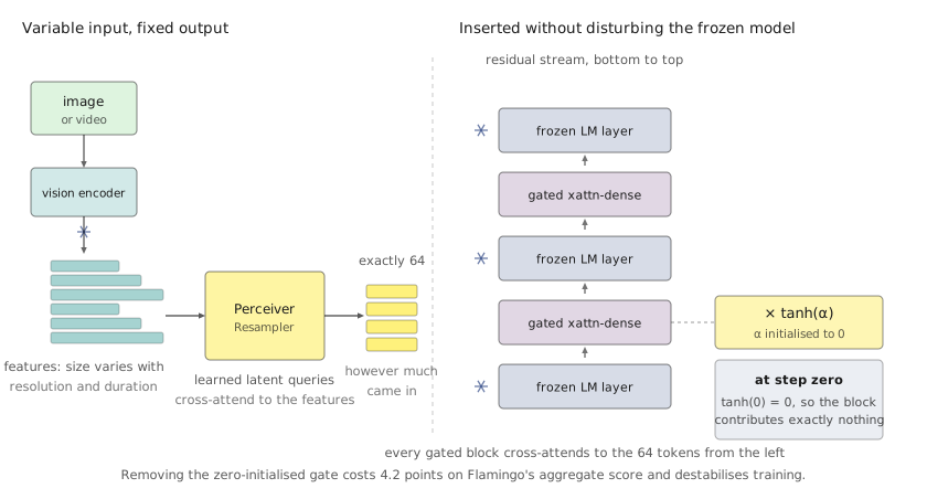
The first problem is quantity. A vision encoder’s output grid varies with resolution, and video makes it worse — frames sampled at one per second turn a clip into a spatio-temporal grid whose size depends on duration. Cross-attention over that is expensive and its cost is unpredictable. Flamingo inserts a Perceiver Resampler, which holds a fixed set of learned latent queries that cross-attend to the visual features and emit a fixed 64 visual tokens no matter how many features came in. Variable-size input, constant-size output, with the compression learned rather than imposed by pooling — and in ablation it beats both a plain transformer and an MLP in that position.

The second problem is the one that dictates the architecture. Flamingo’s language model is a frozen Chinchilla, and freezing it is the point: its few-shot ability is what Flamingo is trying to inherit, and fine-tuning would put that at risk. But new layers initialised at random, inserted between pretrained blocks, corrupt the residual stream immediately — the first forward pass injects noise into representations the frozen model spent its entire training run learning to rely on.

The fix is a gate. Each inserted GATED XATTN-DENSE block multiplies its output by $\tanh(\alpha)$ before adding it to the residual stream, where $\alpha$ is a learnable scalar initialised to zero:

$$y \leftarrow y + \tanh(\alpha_{\text{xattn}}) \cdot \text{attn}(q = y,\; kv = x), \qquad y \leftarrow y + \tanh(\alpha_{\text{dense}}) \cdot \text{ffw}(y). \tag{17.5}$$

Since $\tanh(0) = 0$, the new block contributes nothing at step zero and the conditioned model’s output is identical to the frozen language model’s. Vision does not intrude; it is admitted, gradually, as far as the gradient finds it useful, and each layer sets its own $\alpha$ independently. Removing the zero-initialised gate costs 4.2 points on the aggregate score and destabilises training — this is a load-bearing detail, not a flourish, and the same idea recurs wherever a pretrained network has to be extended without being disturbed.

Figure 17.7: Flamingo’s architecture. The Perceiver Resampler turns a variable-size feature grid into exactly 64 visual tokens; gated cross-attention blocks are interleaved between the frozen language model’s layers, each scaling its contribution by $\tanh(\alpha)$ with $\alpha$ initialised to zero. At initialisation the composite model computes exactly what the frozen language model computes.

The third piece is the training data, and it is what produces the capability the model is remembered for. Flamingo trains on web pages with images and text interleaved in their original order, rather than on isolated image–caption pairs. A sequence therefore looks like several images, each with surrounding prose — which is structurally identical to a few-shot prompt. The attention mask then does something deliberately severe: each text token may attend to the visual tokens of only the single most recent preceding image, not to all images in the sequence. Cross-attention is strictly local; the frozen language model’s own self-attention, which sees the whole sequence, is what carries information across examples.

Figure 17.8: Flamingo’s per-image masking on an interleaved sequence. Each text token cross-attends only to the visual tokens of the image immediately preceding it, so the association between an image and its own text is never diluted. Longer-range structure — the pattern that makes a sequence of examples a few-shot prompt — is carried by the language model’s self-attention, which is unmasked.

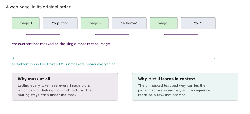
The constraint is what makes the arrangement work. Letting every token attend to every image would blur the image–text correspondence the model needs; forbidding it keeps each pairing crisp while the unmasked text pathway still lets the model recognise that the earlier pairs demonstrate a pattern. Trained this way, Flamingo does in-context learning across modalities: shown three image–answer pairs in a novel format and then a fourth image, it continues the pattern, with no gradient step and no task-specific head. It sets a new few-shot state of the art on 16 benchmarks, and on six of them a few-shot Flamingo surpasses models that were fine-tuned on the full training set — orders of magnitude more task-specific data.

17.8 Open weights are not open data

By 2024 the frontier multimodal models were proprietary, and the open replications shared a dependency that limited how good they could get. Their instruction data came from GPT-4V — the pipeline of Section 17.6, run against a stronger teacher — which is distillation, and a distilled student is bounded by its teacher. It also means the open community’s models improve only when a closed model does, which is a strange position for open research to occupy.

Molmo argues that the gap was never architectural. Its model is deliberately unremarkable: a vision encoder, a connector, a language model, assembled the way Section 17.6 describes. The claim is that the difference between the open models and the closed ones is data, and that the right response is to collect it rather than to distill it.

The difficulty is that the data you want is dense description — long, detailed, exhaustive text about what is in an image — and internet alt-text is the opposite. Alt-text is incidental: it exists to serve some other purpose, it is short, it is often a filename or an SEO fragment, and it describes almost nothing about the image’s actual contents. Asking crowdworkers to type dense captions instead runs into a plain human fact, which is that people will not type for very long, and the captions come back short no matter how the task is worded.

The workaround is the part of Molmo most worth remembering, because it solves an annotation problem by changing the modality of annotation rather than the incentive. Annotators are asked to describe the image out loud for 60 to 90 seconds, and the speech is transcribed. Speaking is fast and low-effort where typing is slow and effortful, and a person who will type twelve words will happily produce two hundred. Prompts direct attention to what a caption normally omits — spatial relationships, counts, text appearing in the image, background detail — and the resulting PixMo-Cap dataset holds 712,000 images with captions far longer than anything scraped. No VLM was involved at any point, so the ceiling is human rather than GPT-4V.

The second dataset is a genuine addition to what these models can do. Grounding — saying where something is — has historically meant bounding boxes or segmentation masks, both slow and awkward to annotate. Molmo asks annotators to point, emitting 2D coordinates, and collects 2.3 million pointing annotations. A point is much cheaper than a box and turns out to be the more useful primitive.

Figure 17.9: Pointing as a single output primitive. The same coordinate output grounds a referring expression, answers a counting question by enumerating instances rather than estimating a number, and hands a target to a downstream system — a segmentation model that turns the point into a mask, or a robot that turns it into a waypoint. Boxes and masks each serve one of these; a point serves all three and is the cheapest of the three to annotate.

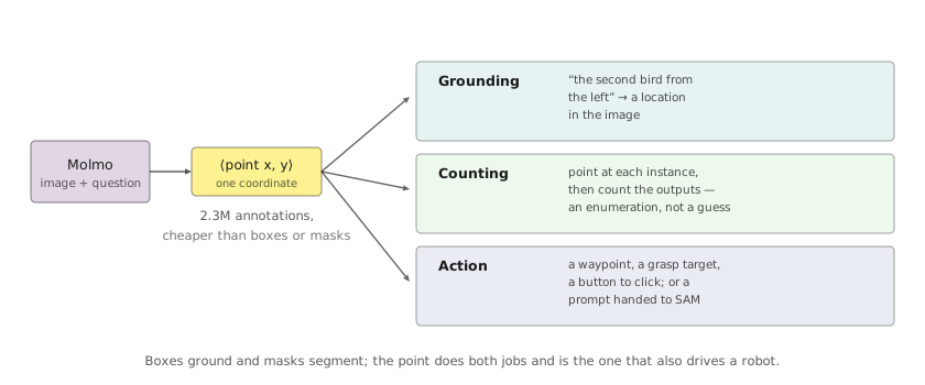
Pointing unifies three things that were separate. It grounds language, by attaching a phrase to a location. It fixes counting: a model asked how many now answers by pointing at each instance and counting its own outputs, which converts a perceptual estimate into an enumeration and is measurably more accurate. And it is an action interface — a point is a navigation waypoint, a grasp target, or a UI element to click, so the same output that answers a question can drive a robot or an agent. A point is also composable with a model that turns points into regions, which is exactly what Section 17.9 provides; chaining the two gives segmentation masks for anything Molmo can name, with neither model trained for the combination.

Molmo’s 72B model ranks second on human-preference evaluation among all models tested, open and closed, and achieves the highest academic benchmark score in its comparison — from a conventional architecture and better data. The lecture’s summary is the correct one: quality over quantity, and intentional collection over incidental scraping, even for pretraining.

17.9 Promptability as the pretraining task

Every model so far outputs text. Segmentation asks for something else — a mask, per pixel — and the question of what a foundation model for segmentation would even be is not obvious, because segmentation has no equivalent of a caption to supervise it at scale.

SAM resolves this by choosing the task first. Rather than segmenting a fixed set of categories, it defines promptable segmentation: given an image and a prompt indicating what to segment — a point, a box, a rough mask, or text — return a valid mask. The prompt vocabulary is open, and the task is general enough to serve both as a pretraining objective and as the interface downstream users get.

Making it work requires confronting a problem that supervised segmentation datasets define away by fiat. A prompt is frequently ambiguous, and irreducibly so. A single point on a person’s shirt might mean the shirt, the person, or the group the person is standing in. All three are correct segmentations of that point, and no amount of additional training data settles which one was intended, because the intent is not in the image. A model forced to emit one mask learns to average the three, which is the worst answer available — a mask that is nobody’s intended object.

SAM’s response is to predict three masks per prompt with a confidence score each, corresponding roughly to the part, the whole, and the containing group. During training the loss is computed against the best-matching of the three only, so the three heads specialise rather than converging; at inference the caller picks. Ambiguity is represented rather than resolved.

Figure 17.10: SAM’s architecture, drawn along the axis that its runtime behaviour depends on. The heavy ViT encoder runs once per image and its embedding is reused; each prompt then costs only the lightweight decoder, which is why interactive use with many prompts stays real-time. The decoder emits three masks with confidence scores, so an ambiguous point returns the part, the whole and the group rather than an average of them.

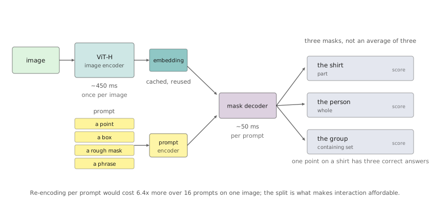
The cost structure in Figure 17.10 is a design decision, not a consequence. Interactive segmentation means many prompts against one image — a user clicking repeatedly, or a downstream model probing a grid of points — and the asymmetry between a heavy encoder run once and a tiny decoder run per prompt is what makes that affordable. Encode once, decode cheaply, many times.

That leaves the data, and here the promptable task pays for itself in a way worth following, because the model and the dataset are built by the same process. There is no web-scale source of segmentation masks the way there is for image–text pairs, so SAM’s authors ran a data engine in three stages. First, annotators segment interactively with model assistance, and the model retrains on what they produce. Then the model proposes confident masks itself and annotators only fill in what it missed, which shifts human effort towards the model’s blind spots. Finally, the model annotates fully automatically: prompted with a dense grid of points across each image, filtered for confidence and stability, it generates masks with no human in the loop. The result, SA-1B, holds over 1 billion masks across 11 million images — roughly 400 times more masks than any prior segmentation dataset — and the great majority were produced by the model the dataset was collected to train. Each stage’s model makes the next stage’s annotation cheaper, and the loop is only possible because the task was defined to be promptable in the first place.

What SAM does not do is name anything. It segments what you point at and has no notion of what the region is, which is precisely why it composes so well with the models of the previous sections: CLIP or Molmo supplies the semantics and the location, SAM turns the location into a boundary. Neither was trained for the pairing.

17.10 Chaining, and the case for not training

Everything above answers a new demand by training something. There is a fourth move, and by the end of the lecture it is the one that looks most like where the field went: leave the models frozen and compose them.

The small version of the idea is CuPL, which revisits the prompts of Section 17.3. Those templates are hand-written, generic, and identical for every class — a photo of a {label} says nothing about what distinguishes the label from anything else. But a language model has read a great deal about these categories and knows what they look like. So CuPL asks one: what does a platypus look like? The answers come back as descriptive sentences naming the discriminating features — the bill, the flat tail, the fur — and those sentences become the prompts. The classifier’s weights are now written by a model that knows something about the class, rather than by a template that knows only its name. It gains over a percentage point on ImageNet, requires no training and no hand-written templates, and its ingredients are two frozen models and a prompt.

VisProg generalises the move as far as it goes. Given a natural-language instruction — something compositional, of the kind a single model handles poorly, like tag the seven dwarfs in this image or hide the face of the person on the left — it uses a language model’s in-context learning to emit a short Python-like program. Each line calls a module: an object detector, CLIP, a segmentation model, an inpainting model, an image-processing routine, or plain arithmetic. An interpreter then executes the program line by line, feeding each module’s output to the next.

Figure 17.11: VisProg’s execution. A language model, given a few examples of instruction-and-program pairs, compiles a new instruction into a short program over frozen modules; an interpreter runs it, threading intermediate results through. Nothing is trained — extending the system to a new capability means registering a module and adding an example to the prompt — and the program itself is the explanation of how the answer was produced.

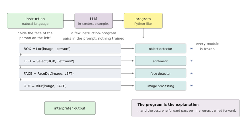
Nothing is trained. The language model has never been fine-tuned for this; it is shown a handful of instruction-and-program pairs in context and generalises to new instructions from there. Adding a capability means registering a module and adding one example to the prompt, which is a considerably shorter path than collecting a dataset. And the interpretability is genuine rather than post-hoc: the program is the reasoning, the intermediate outputs can be inspected at every line, and when the answer is wrong you can see which step produced the wrong thing.

The costs are real and the lecture states them. Every module invocation is a full forward pass, so latency compounds down the program; if any module is a hosted API, each line is a paid call and a network round trip. Errors compound too, since a mistake early in the program is faithfully propagated by every step after it, and the system has no way to notice. Composition buys flexibility and interpretability at the price of speed and reliability.

17.11 What the chapter adds up to

The trajectory here has a shape, and it is worth naming because it is not the shape one would guess from the architectures alone. Nothing in this chapter turned on a new layer type. CLIP is a contrastive loss the field already had, pointed at a supervision signal that was already lying on the internet. LLaVA is a matrix. Flamingo’s one real invention is a scalar initialised to zero. Molmo’s architecture is conventional by design, and its contribution is a microphone. SAM’s is a task definition that makes its own dataset collectable. VisProg trains nothing at all.

What each of them changed instead was the interface. CLIP replaced a fixed label set with an open vocabulary, at the cost of a representation too coarse to say where anything is or how many there are. LLaVA and Flamingo replaced a similarity score with free-form text, by two different routes — concatenate into the prompt, or cross-attend through a gate — and the choice between them comes down to whether the language model may be modified. Molmo replaced the caption with the point, which grounds, counts, and acts through one output. SAM replaced the category with the prompt. And chaining replaced the model with a program over models.

The limitation from Section 17.5 survives all of it, which is the note to end on rather than a summary. A model trained to rank captions against random negatives learns which words are present and not how they compose, and every downstream system in this chapter inherits some of that. Better data narrows it, generative objectives narrow it, explicit programs route around it — but the compositional structure of a visual scene is still the thing these models represent least well, and it is the thing the next chapter’s robots cannot do without.