16  3D Vision

Lecture 15

Based on Lecture 15 of CS231n, Stanford University, Spring 2025, given by Jiajun Wu.

16.1 The question images never ask

Everything in the preceding fourteen chapters rested on a convention so uniform that it never had to be argued for. An image is a grid of pixels. Two hundred by two hundred, three channels, row-major; a JPEG and a PNG disagree about compression and agree completely about what they are compressing. Convolution assumes that grid, pooling assumes it, patch embedding assumes it, and the entire apparatus of transfer learning works because every image anyone has ever trained on is the same kind of object as every other.

Geometry has no such convention, and the absence is not an oversight waiting to be corrected. A shape can be handed to you as a few hundred thousand points scraped off a laser scanner, as a mesh of triangles with a texture atlas, as a solid assembled from cylinders and boxes by Boolean operations in a CAD kernel, as the zero level set of a function, or as the weights of a neural network that answers queries about occupancy. These are not five encodings of one canonical object in the way that PNG and JPEG are. They support different operations, they fail in different places, and converting between them loses something every time.

The lecture opens by listing what a representation is being asked to do, and the list is longer than it first appears. It has to be stored, which for a pixel grid is a matrix and for an irregular point set is already a question. It has to support creation — someone or something has to author new shapes, whether that is an artist with a mouse, a scanner, or a generative model conditioned on a sentence. It has to support operations: editing, smoothing, simplification, repair, the whole toolbox that a shape passes through between capture and use. It has to render, turning geometry back into pixels, and this one matters more than the others for our purposes, because rendering is the bridge that lets two-dimensional data supervise three-dimensional models. And for anything that moves — humans, animals, articulated machines — it has to animate, which means the representation has to survive being deformed.

No single choice is good at all five. That is the whole reason the taxonomy exists rather than a winner, and it is why a chapter on 3D vision has to spend its first half on geometry before it can spend its second half on learning. The deep-learning results in Section 16.7 onwards are not a sequence of architectures. They are a sequence of bets on representation, and each one is legible only against the map that the classical literature drew first.

16.2 Points, and what they cannot tell you

A point cloud is an unordered set of coordinates in $\mathbb{R}^3$, and it is the simplest thing that can be called a shape. Where an image is an $n \times n$ matrix whose entries are indexed by position, a point cloud is a $3 \times n$ matrix whose columns are positions and whose column order carries no information at all. That last clause is doing more work than it looks like; Section 16.9 is entirely about its consequences.

Points are what sensors produce. A structured-light depth camera, a lidar unit, a photogrammetry pipeline, the scanner in a modern phone — all of them emit points, possibly noisy, usually in the sensor’s own frame, and getting a single coherent cloud out of several passes is the registration problem. Each point may carry a surface normal alongside its position, in which case it is called a surfel: a position with an orientation. The normal is not decoration. Shading a surface requires knowing how it faces the light, so a cloud without normals can be plotted but not convincingly rendered.

The appeal is that points constrain nothing. Any geometry at all can be approximated by enough of them, at any scale, with no requirement that the shape be closed, connected, or of any particular topology, and adding detail in one region is a matter of putting more points there. The price is that a set of positions is less than a surface, and the shortfall is precisely topological. Given a ring of points, there is no way to tell whether they were sampled from a torus or from a circle of disconnected beads; the samples are identical and the connectivity that would distinguish them was never recorded. Nothing in the representation says which points are neighbours, so the operations that depend on neighbourhood — subdividing, simplifying, smoothly interpolating between samples — have nowhere to start. They can be recovered, at a cost, by imposing a spatial data structure and estimating neighbourhoods from proximity, which is exactly what the point-cloud networks of Section 16.9 quietly spend their capacity on.

The polygonal mesh is the answer to that shortfall, and it is the representation the rest of the graphics world runs on. Keep the vertices, and add faces: a list saying which vertices bound each polygon. This is a boundary representation — the surface of the object is stored, the interior is implied — and it converts a cloud into a piecewise-linear surface with a well-defined inside, a well-defined normal per face, and an explicit notion of adjacency. Meshes scale to essentially any size. The Digital Michelangelo Project’s scan of the David carries $28{,}184{,}526$ vertices and $56{,}230{,}343$ triangles, and Google Earth’s reconstruction of the planet from satellite and aerial imagery runs to trillions.

What connectivity buys is the toolbox. Subdivision raises resolution by inserting vertices according to a fixed rule, so a coarse control mesh can carry fine detail without an artist placing every vertex. Simplification goes the other way, collapsing edges to reduce triangle count while preserving silhouette and appearance, which is how a game engine draws a distant object cheaply. Regularisation redistributes vertices so that triangles are near-equilateral and roughly uniform in size, because almost every downstream algorithm behaves better on a well-conditioned mesh than on a mesh with slivers. None of these three has a natural analogue on a raw point cloud, and all three are immediate once faces exist.

The same connectivity is what made meshes awkward for early deep learning. A raw mesh is irregular in two separate ways: different faces may have different numbers of vertices, and different meshes have different numbers of faces. A convolutional network of the era wanted a fixed-resolution grid, and a mesh is not one. This is a large part of why deep learning arrived in 3D vision several years after it had settled everything in 2D — not because the ideas did not transfer, but because there was no agreement on what the network should consume.

16.3 Surfaces as maps

Points and meshes are both non-parametric: they store samples, and the number of numbers grows with the amount of detail. But a great deal of real geometry is not arbitrary. The intrinsic dimensionality of a curve is one and of a surface is two, whatever ambient space they sit in, and a manufactured object is usually built from pieces that were specified by a designer rather than measured off a scanner. A parametric representation exploits both facts by storing the map instead of the samples.

The pattern is to name a low-dimensional domain and a function out of it. A circle in the plane is the image of an interval,

$$\gamma(t) = (\cos t, \sin t), \qquad t \in [0, 2\pi), \tag{16.1}$$

and a sphere in space is the image of a rectangle under the two angles of latitude and longitude. In both cases the shape is the range of a function: the parameters are the true degrees of freedom, and the function is what carries them into $\mathbb{R}^3$. Nothing is sampled until someone asks for a point.

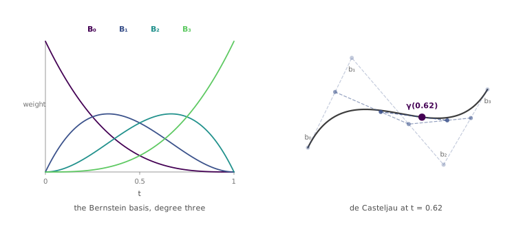
Trigonometric formulas cover the shapes that happen to have them, which is not many. The workhorse of design is instead a family of polynomial maps controlled by a handful of points that an artist can drag. A Bézier curve of degree $n$ is a weighted average of $n+1$ control points $\mathbf{b}_0, \dots, \mathbf{b}_n$, where the weights are the Bernstein polynomials:

$$\gamma(t) = \sum_{i=0}^{n} \binom{n}{i} (1-t)^{n-i} t^{i} \, \mathbf{b}_i , \qquad t \in [0,1]. \tag{16.2}$$

The weights are non-negative and sum to one for every $t$, which is why the curve never escapes the convex hull of its control points — the property that makes the control polygon a usable interface. The same expression can be evaluated without ever writing a binomial coefficient, by de Casteljau’s algorithm: repeatedly linearly interpolate along the control polygon,

$$\mathbf{b}_i^{(k)}(t) = (1-t)\,\mathbf{b}_i^{(k-1)}(t) + t\,\mathbf{b}_{i+1}^{(k-1)}(t), \tag{16.3}$$

starting from $\mathbf{b}_i^{(0)} = \mathbf{b}_i$ and stopping when a single point $\mathbf{b}_0^{(n)}(t) = \gamma(t)$ remains. That the recursion and Equation 16.2 agree is not obvious from the two expressions, and the generator behind Figure 16.1 checks it numerically rather than taking it on faith.

Surfaces follow by taking the tensor product. Run a Bézier curve in $u$ whose control points are themselves the values of Bézier curves in $v$, and the result is a Bézier patch governed by a $4 \times 4$ grid of control points for the bicubic case; a complicated object is then a quilt of patches joined with matching tangents at their seams. This is the machinery underneath the spline and NURBS surfaces that CAD systems use, and it is why a designed object can be edited long after it is authored: moving one control point changes the surface smoothly and locally, which is not true of moving one vertex of a dense mesh.

Figure 16.1: Two routes to the same cubic Bézier curve. Left, the Bernstein weights of Equation 16.2 as functions of $t$; right, the de Casteljau construction of Equation 16.3 at $t = 0.62$, where each round of linear interpolation shrinks the control polygon by one vertex until a single point is left on the curve. The generator evaluates both forms on a dense grid and asserts they agree to machine precision.

Subdivision sits between the parametric and non-parametric worlds and is worth seeing as the limit of a rule rather than as a formula. Chaikin’s corner-cutting scheme takes a polygon and replaces every edge by the two points one quarter and three quarters of the way along it, discarding the original vertices; iterate, and the polygons converge to a quadratic B-spline. The surface analogues — Catmull–Clark, Loop — do the same thing to a mesh, and they give an artist a coarse control cage whose refinement is smooth by construction. The representation stored is discrete; the object it denotes is the limit.

16.4 The asymmetry that organises everything

Points, meshes, splines and subdivision surfaces differ in almost every respect and agree on one: they all hand you points. Sample the parameters, evaluate, and you have a location that is on the surface by construction. This is what makes them explicit. The alternative is to give up direct access to the points and instead state a condition that the points on the surface satisfy — to define the shape as the set where some function vanishes,

$$S = \{\, \mathbf{x} \in \mathbb{R}^3 : f(\mathbf{x}) = 0 \,\}, \tag{16.4}$$

which is an implicit representation. The unit sphere is $f(\mathbf{x}) = x^2 + y^2 + z^2 - 1$, and nothing about that expression tells you a single point on the sphere.

The contrast is sharpest when the same object is written both ways. A torus is the image of a square under

$$f(u, v) = \big((2 + \cos u)\cos v,\ (2 + \cos u)\sin v,\ \sin u\big) \tag{16.5}$$

and it is also the zero set of

$$g(x, y, z) = \Big(2 - \sqrt{x^2 + y^2}\Big)^{2} + z^{2} - 1 . \tag{16.6}$$

Ask each for a hundred points on the surface. The explicit form answers by drawing a hundred $(u, v)$ pairs and evaluating — a hundred function calls, every answer exact. The implicit form has to solve $g = 0$, an equation in three unknowns with a two-dimensional solution set, and for Equation 16.6 that is still tractable by hand while for an arbitrary $g$ it is a root-finding problem with no closed form at all.

Now ask each whether the point $(3/4,\, 1/2,\, 1/4)$ lies inside the corresponding sphere. The implicit form evaluates its function once:

$$f\!\left(\tfrac{3}{4}, \tfrac{1}{2}, \tfrac{1}{4}\right) = \tfrac{9}{16} + \tfrac{4}{16} + \tfrac{1}{16} - 1 = -\tfrac{1}{8} < 0,$$

so the point is inside, since $f$ is negative within the shape, zero on it and positive outside. The explicit form has no comparable move. A parameterisation is a map out of the domain; it offers no way to run backwards from an arbitrary query point, and deciding containment means something like casting a ray and counting crossings of the surface — a global computation, not an evaluation.

The two representations are therefore not ranked. They are exactly opposed, and it is worth stating the opposition plainly because everything in the rest of this chapter is a consequence of it.

	Explicit	Implicit
Sample a point on the surface	evaluate the map — trivial	solve $f = 0$ — hard
Test whether a query point is inside	global computation — hard	evaluate $f$ once — trivial
Compose two shapes	remesh the intersection	arithmetic on the two functions
Storage grows with	the amount of detail stored	the complexity of $f$

Figure 16.2: The same asymmetry on the same two objects. Sampling the surface is one evaluation of the explicit map and a root-find for the implicit function; testing containment is one evaluation of the implicit function and a ray cast for the explicit map. Neither representation is better; each is the other’s complement.

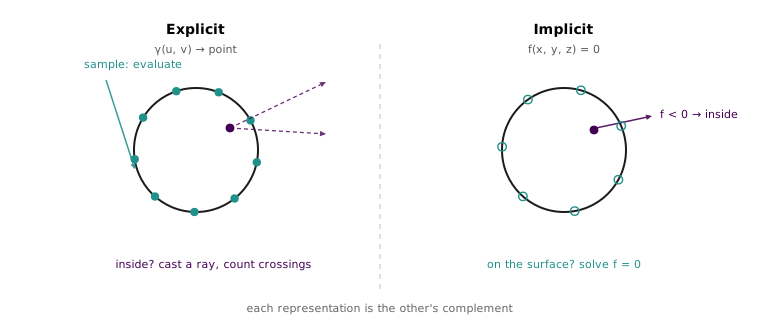
Which query a method needs is what decides its representation, and the reason this section is load-bearing is that the query changed. Classical geometry processing mostly wanted to sample surfaces, which is why explicit forms dominated for thirty years. Neural rendering wants to ask, of an arbitrary point in space, what the density is there, what the colour is, what the material is — the containment query, repeated millions of times per image. That shift is the single best explanation for why implicit representations, a niche of CAD and level-set methods in 2010, became the default in 3D deep learning by 2020.

16.5 Building shapes out of functions

An implicit function need not be pulled out of the air. The simplest family is the algebraic surfaces, zero sets of polynomials, which gives spheres, ellipsoids, cylinders, quadrics and the occasional decorative quartic and then runs out of usable expressions long before it reaches anything one would want to manufacture. Nobody writes down the polynomial whose zero set is a cow.

What rescues the implicit view is that its shapes compose arithmetically. If $f$ and $g$ are the functions of two solids under the sign convention that negative means inside, then

$$f \cup g = \min(f, g), \qquad f \cap g = \max(f, g), \qquad f \setminus g = \max(f, -g), \tag{16.7}$$

and each of these is a one-line operation on values rather than a geometric construction. This is constructive solid geometry, and it is how mechanical CAD has worked for decades: a part is a tree whose leaves are primitives and whose internal nodes are Booleans, and the whole tree is evaluated at a query point by evaluating the leaves and folding upwards. Doing the same thing to two meshes means computing the surface of intersection, splitting triangles along it and repairing the result — a notoriously fragile operation that implicit geometry gets for the price of a comparison.

Booleans give hard creases. Something smoother is available when the function carries more information than its sign, and the natural choice is the signed distance function, whose value at $\mathbf{x}$ is the distance from $\mathbf{x}$ to the surface, negative inside:

$$d(\mathbf{x}) = \pm \min_{\mathbf{y} \in S} \lVert \mathbf{x} - \mathbf{y} \rVert . \tag{16.8}$$

Now the magnitudes mean something, so shapes can be averaged rather than merely combined: interpolating between two distance fields moves a boundary continuously from one shape to the other, and softened variants of Equation 16.7 blend two solids into a fillet instead of a crease. Practitioners of the technique compose dozens of such fields into entire rendered scenes, and the reason it is practical at all is that a distance field also tells a ray marcher how far it may safely step — the value at the current point is a radius within which no surface can lie.

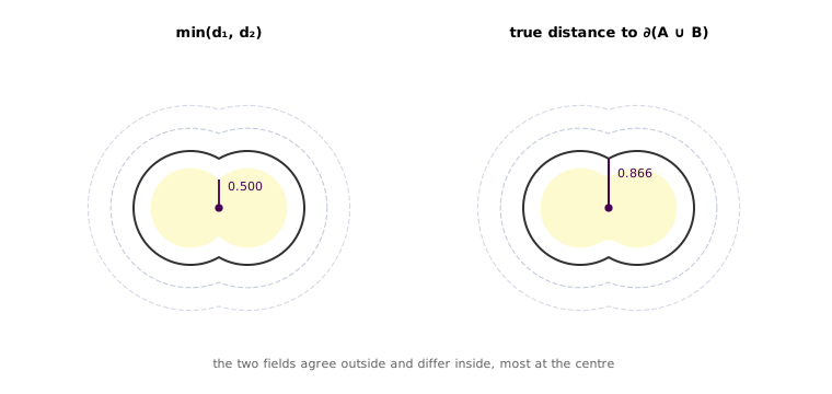
That last property is where the lecture’s presentation of Equation 16.7 is worth pushing on, because the identity is exact in one place and only a bound in another. Take two overlapping unit disks with centres at $(\pm\tfrac{1}{2}, 0)$ and query the origin. Each disk reports $d = -\tfrac{1}{2}$, so $\min$ reports $-\tfrac{1}{2}$; the true distance from the origin to the boundary of the union is $\sqrt{3}/2 \approx 0.866$, because the arcs that ran nearest the origin are interior to the other disk and no longer part of the boundary at all. Outside the union the two agree exactly, and inside it $\min$ systematically understates the depth. The composition rules are therefore safe for the thing ray marchers use them for — stepping in from outside — and are not a true distance function on the interior, which is why implicit-surface code that needs interior distances recomputes rather than composing. The generator behind Figure 16.3 evaluates $\min(d_1, d_2)$ against a brute-force distance to the union’s boundary over a grid and reports the largest discrepancy on each side of the surface, so the claim is measured rather than remembered.

Figure 16.3: The signed distance fields of two overlapping disks and of their union. Contours are level sets of the field, and the heavy contour is the surface itself. Outside the union, $\min(d_1, d_2)$ reproduces the true distance exactly; inside it, the arcs swallowed by the other disk are no longer boundary, so the composed field understates the true depth — largest at the centre, where it reports $0.5$ against a true $0.866$.

Composition still leaves the problem that a complicated object needs a large expression tree, and evaluating hundreds of primitives per query is slow. The fix is to give up the closed form and precompute: lay a regular grid over the domain, evaluate the function once at every node, and store the values. The surface is then recovered wherever interpolated values cross zero, which for a grid means wherever two adjacent samples have opposite sign. This is the level-set representation, and it is what medical imaging has always produced — a CT or MRI volume is a scalar field, and an isosurface of constant tissue density is a shape extracted from it exactly this way.

Discard the magnitudes and keep only the sign and the level set collapses into voxels: a three-dimensional array of occupancies, one bit or one probability per cell. The lecture arrives at voxels by this route deliberately, because the usual route obscures what they are. Presented as “pixels with one more index”, a voxel grid looks like the obvious first thing to try and its costs look incidental. Presented as a sampled implicit function, it is visibly an approximation that has thrown away both the closed form’s exactness and the distance field’s magnitudes, and the only thing it has bought in exchange is a regular array. That purchase turns out to matter enormously, because a regular array is what a convolution wants.

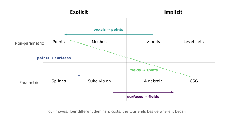
Every representation in this chapter’s first half now has a place on a single map, and the map is the object the rest of the chapter moves around. One axis is the explicit–implicit distinction of Section 16.4. The other is whether the shape is stored as samples or as a function of a few parameters.

Figure 16.4: The taxonomy the lecture builds, with the four moves that the deep-learning literature made across it. Voxels were the first target because they are the only cell a convolution can be run on unchanged; each later move is a bet that some other cell suits the query better.

16.6 What there was to learn from

Methods in 3D lagged 2D by several years, and part of that was the representation problem of Section 16.2. The rest was data. The standard benchmark before deep learning was the Princeton Shape Benchmark of 2004: $1{,}814$ models across $182$ categories, which is about ten examples per class. It was considered large. Ten examples per class is not a training set under any modern reading; it is an evaluation set for methods that learn nothing.

The change came from the same place it came from in 2D — someone assembled a corpus large enough that learning became the obvious thing to do. ShapeNet indexed more than three million models from online repositories, of which $220{,}000$ were sorted into $3{,}135$ categories, and released ShapeNetCore, a clean subset of $51{,}300$ models in $55$ categories that became the benchmark for essentially every method in the second half of this chapter. The scale-up did not stop: Objaverse collected $818{,}000$ artist-made assets, and Objaverse-XL roughly $10.2$ million, drawn mostly from GitHub and Thingiverse.

Synthetic assets have a specific weakness. They are what someone chose to model, which means clean topology, canonical poses, plausible materials and no sensor noise — the distribution of CAD files, not of objects. So a second lineage grew alongside it, made of scans. CO3D contains nearly $19{,}000$ turntable-style videos of objects in $50$ MS-COCO categories, $1.5$ million frames with camera poses attached. ScanNet does the same for interiors: $2.5$ million RGB-D views across $1{,}513$ scans, with poses, reconstructed surfaces and instance-level semantic labels, later extended by ARKitScenes and ScanNet++. A third lineage annotates below the object: PartNet labels $573{,}585$ fine-grained part instances across $26{,}671$ shapes in $24$ categories, hierarchically and with mobility, which is the data that Section 16.14 needs and that nothing else supplies.

Figure 16.5: 3D corpora by size and year, on a logarithmic axis, against ImageNet for scale. Four orders of magnitude in twenty years, and still roughly one order short of the 2D corpora that pretrained models are built on — which is the practical case for supervising 3D models through rendering rather than through 3D labels.

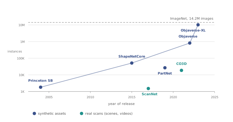
The comparison to draw from Figure 16.5 is not that 3D data grew, but where it ended up. Objaverse-XL is a genuinely large corpus and it is still smaller than ImageNet, and smaller by a wide margin than the billion-image sets behind current 2D foundation models. The scanned datasets, which carry the realism, are three to four orders below that. Any method that needs 3D supervision is therefore working in a regime that 2D vision left behind a decade ago, and this is the standing argument for the recurring move in the rest of the chapter: put a differentiable renderer between the 3D model and the loss, and supervise it with photographs, of which there are effectively unlimited numbers.

16.7 Sidestepping the problem: render it first

The first serious attempt to run a network on shapes did not solve the representation problem. It avoided it.

Multi-view CNN places a ring of virtual cameras around the object, renders one image per camera, and hands each image to an ordinary image network — the same architecture, initialised from the same ImageNet weights, that had just finished winning everything in 2D. The per-view features are combined by view pooling, an element-wise maximum across the views, and the pooled descriptor goes through a second convolutional stage and a softmax. The max is what makes the design work: it is invariant to which view is which, so the network produces one descriptor per shape rather than one per camera, and the shape can be classified or retrieved from that descriptor alone.

Figure 16.6: Multi-view CNN. Each rendered view goes through the same weights, an element-wise maximum over views collapses them into a single order-independent descriptor, and a second stage classifies it. The maximum is the whole architectural idea: everything before it is an ordinary image network, and everything after it sees a shape rather than a picture.

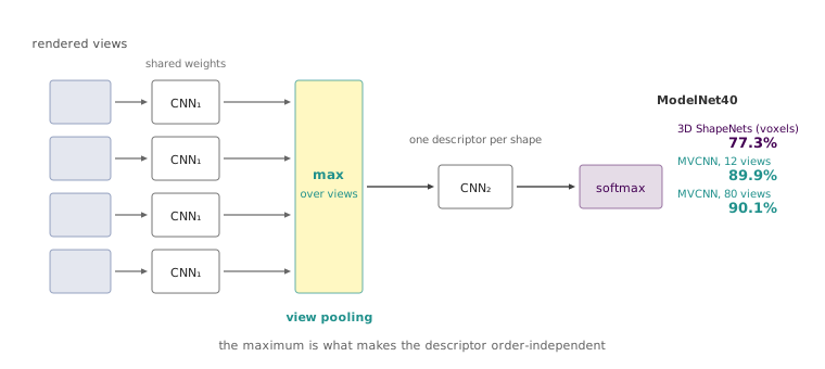
On ModelNet40 the results were not close. The best learned 3D descriptor of the day, the voxel-based 3D ShapeNets, reached $77.3\%$ classification accuracy and $49.2\%$ retrieval mAP. Twelve rendered views through an ImageNet-pretrained network reached $89.9\%$ and $70.1\%$; going to eighty views moved classification only to $90.1\%$, so the gain came from rendering at all rather than from rendering exhaustively. The paper’s sharpest observation is stranger still: a network trained on the twelve views but shown a single view at test time already beat the 3D methods by about eight points. Whatever the voxel networks were learning about three-dimensional structure was worth less than what an ImageNet-pretrained 2D network already knew about surfaces, materials and silhouettes.

The lesson is about data, not about geometry, and it is the direct consequence of Figure 16.5. A projection throws away most of the shape; what it buys in return is access to a pretraining corpus three orders of magnitude larger. In 2015 that trade was overwhelmingly favourable. The field then spent a decade building native 3D methods on the argument that it would stop being favourable as 3D corpora grew — and the lecturer’s aside is that with current image and video foundation models the trade may be swinging back, which is a live question rather than a settled one.

Multi-view has two genuine weaknesses that the accuracy numbers hide. It needs a renderable input, so a noisy or partial point cloud has to be reconstructed before it can be photographed, and reconstruction is the hard problem it was supposed to avoid. And its output is a descriptor, not geometry: the pipeline classifies and retrieves, but it cannot produce a shape.

16.8 Voxels, and the exponent they pay

The obvious native alternative was the one that required changing a single line. Voxels are a dense array, so a convolution runs on them unchanged, and the entire 2D toolkit transfers by replacing every 2D operator with its 3D counterpart. 3D ShapeNets did this with a convolutional deep belief network in 2015, generating and classifying shapes at low resolution; 3D-GAN followed by mapping a $200$-dimensional latent vector through a volumetric generator to a $64^3$ occupancy cube, trained adversarially exactly as in Section 15.2 with every 2D operation swapped for a 3D one.

The interesting move came next, and it is the first appearance in this chapter of the rendering bridge. Visual Object Networks factor generation into three codes — shape, viewpoint, texture — and place a differentiable projection between the first two and the third: the generated voxel shape is rendered from the sampled viewpoint into a depth map and a silhouette, and a second network paints that geometry into a colour image. Two adversarial losses then apply, one demanding that the 3D shapes look like real shapes and one demanding that the 2D renderings look like real photographs. Because the three codes enter at different points, they stay disentangled, so viewpoint, geometry and appearance can be varied independently and a texture can be transferred from one car onto the shape of another. This is the pattern that Section 16.12 makes the centre of the field: the renderer is the thing that lets abundant 2D data supervise scarce 3D structure.

What limits all of it is arithmetic. A voxel grid at resolution $n$ costs $O(n^3)$ memory and compute, while the object it represents is a surface, whose area grows as $O(n^2)$. The ratio is the fraction of cells that carry any information at all, and it falls like $1/n$: almost every cell in a fine grid is either empty space or buried interior, and the network spends the overwhelming majority of its capacity convolving nothing with nothing. Doubling resolution costs eight times the memory to gain four times the surface detail.

Octrees recover the exponent. Partition the cube into eight children, and recurse only into the children that the surface actually crosses; cells far from the surface stay large. The stored structure is then proportional to the surface rather than the volume, which restores $O(n^2)$ scaling, and specialised convolution implementations — OctNet, O-CNN — run directly on the tree. For generation the trick is subtler, because the tree’s structure is not known in advance: Octree Generating Networks predict the octree layer by layer, deciding at each level which cells are empty, filled, or mixed and therefore worth subdividing, and only the mixed cells are expanded at the next level. That buys output volumes as large as $512^3$ in a single forward pass on hardware where a dense decoder had been stuck near $64^3$.

Figure 16.7: Why the exponent matters. A dense grid costs $O(n^3)$ cells while the surface it represents occupies $O(n^2)$ of them, so the occupied fraction falls as $1/n$: counting the cells a sphere’s boundary actually crosses gives $19.3\%$ at $16^3$ and $0.72\%$ at $512^3$, halving at each doubling to within a few percent. The octree curve counts the nodes a surface-following subdivision actually creates. Both curves are computed by the generator, not traced from a published chart.

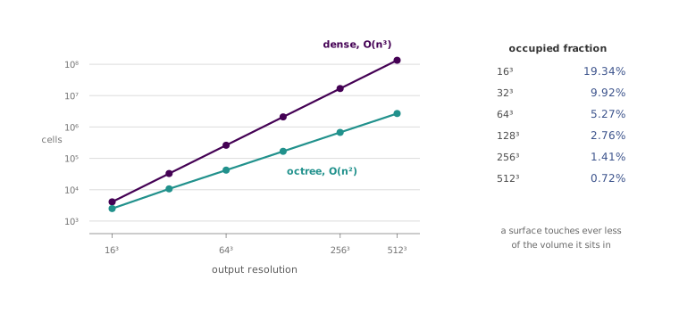
An octree is still a sampled implicit function; it has only stopped sampling uniformly. The next move is a bigger one — abandoning the grid entirely.

16.9 Learning on sets: PointNet

Voxels and octrees both discretise space and record what is in it. Points discretise the object and let it sit wherever it likes. The lecture labels the difference with the terminology of fluid mechanics — Eulerian versus Lagrangian — and it is exactly right: a voxel grid is a fixed lattice of observers reporting what passes through, and a point cloud is a set of particles carrying their own coordinates.

Running a network on the Lagrangian view means confronting the property that Section 16.2 flagged. A point cloud is a set. Reorder the columns of the $3 \times n$ matrix and the shape is unchanged, so the network’s output must be unchanged too, for all $n!$ orderings. A convolution has no such invariance; feeding a point cloud to an MLP in matrix order gives a network that must learn the invariance from data, which for $n = 1024$ is hopeless. PointNet was the first architecture to build it in.

The requirement is that the network compute a symmetric function of its inputs: one whose value is unchanged under any permutation. Familiar examples are the maximum, the sum and the mean, and each is symmetric because it aggregates without reference to position. Applying one directly to the raw coordinates does work and is useless — the element-wise maximum over a point cloud returns a corner of its bounding box, and nothing about the shape survives. The insight is that a symmetric aggregator becomes expressive if the points are transformed first and the aggregate is transformed after:

$$f(\{\mathbf{x}_1, \dots, \mathbf{x}_n\}) \;=\; \gamma\Big( \max_{i=1,\dots,n} h(\mathbf{x}_i) \Big), \tag{16.9}$$

where $h$ is a multilayer perceptron applied to each point independently with shared weights, the maximum is taken element-wise over the $n$ resulting feature vectors, and $\gamma$ is a second perceptron on the pooled result. Composing a symmetric function with anything applied per-point leaves it symmetric, so Equation 16.9 is permutation-invariant by construction rather than by training. What makes it more than a trick is the accompanying theorem: any continuous set function — continuous with respect to Hausdorff distance on sets — can be approximated arbitrarily well in this form, provided the pooled feature vector is wide enough. The maximum is not a lossy shortcut forced on the architecture by symmetry. It is sufficient.

Figure 16.8: PointNet. Every point passes through the same weights, so the network is blind to input order before pooling; the element-wise maximum then reduces $n$ feature vectors to one global descriptor regardless of $n$. Applying the maximum to raw coordinates instead of features would return a corner of the bounding box, which is why the per-point lift comes first.

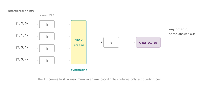
The same design has a visible weakness. A global maximum discards which features came from which points and where those points were relative to each other, so Equation 16.9 has no local receptive field at all — it is a bag of points, and the analogue of a convolution’s locality has to be added back. PointNet++ does it by applying the same construction hierarchically over nested neighbourhoods; dynamic graph CNNs do it by building a $k$-nearest-neighbour graph over the points and passing messages along its edges, recomputing the graph in feature space at each layer so that “neighbouring” comes to mean semantically rather than spatially close. Both restore locality without giving up permutation invariance, because a graph over a set is itself order-independent.

16.9.1 Comparing two sets

A network that outputs a point cloud has a second version of the same problem. The prediction is a set and the target is a set, and a per-element squared error would compare the $i$-th predicted point to the $i$-th ground-truth point, which is meaningless when neither ordering carries information. The loss has to be permutation-invariant too, and the Point Set Generation Network introduced the two that the field has used ever since.

The Chamfer distance matches every point to its nearest neighbour in the other set, in both directions:

$$d_{\mathrm{CD}}(S_1, S_2) = \sum_{\mathbf{x} \in S_1} \min_{\mathbf{y} \in S_2} \lVert \mathbf{x} - \mathbf{y} \rVert_2^2 \;+\; \sum_{\mathbf{y} \in S_2} \min_{\mathbf{x} \in S_1} \lVert \mathbf{x} - \mathbf{y} \rVert_2^2 . \tag{16.10}$$

Each nearest-neighbour search is independent of the others, so the whole thing is trivially parallel and accelerable with a k-d tree, and it is continuous and piecewise smooth in the point positions. It is also not a metric — the triangle inequality fails — and, more consequentially, the matching is not one-to-one. Many predicted points may share a single nearest target, which means a model can leave regions of the target uncovered while every one of its own points sits comfortably close to something.

The Earth Mover’s distance closes that hole by insisting on a bijection between two sets of equal size:

$$d_{\mathrm{EMD}}(S_1, S_2) = \min_{\phi : S_1 \to S_2} \sum_{\mathbf{x} \in S_1} \lVert \mathbf{x} - \phi(\mathbf{x}) \rVert_2 , \tag{16.11}$$

with $\phi$ ranging over bijections. Every predicted point is spent on exactly one target point, so nothing can be double-counted and no region can be quietly abandoned. The cost is that Equation 16.11 is an assignment problem rather than a search, far too expensive to solve exactly inside a training loop, so implementations use a $(1+\epsilon)$-approximation with a fixed time budget per instance. It is differentiable almost everywhere, since the optimal assignment is generically unique and locally constant under small movements of the points.

Figure 16.9: Chamfer against Earth Mover’s on the same pair of sets. Chamfer’s arrows are independent nearest-neighbour lookups, so several predictions can collapse onto one target and leave a target unmatched; the Earth Mover’s assignment is a bijection and every target is claimed exactly once. The matchings are computed by the generator — nearest-neighbour for one, an exact optimal assignment for the other.

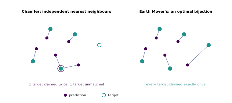
The practical summary is that Chamfer is cheap and tolerant of density mismatch, EMD is expensive and enforces coverage, and a model trained on Chamfer alone tends to produce clouds that score well while sparing themselves the difficult parts of the shape.

16.10 Predicting a surface instead of a cloud

A generated point cloud is still non-parametric, and it inherits everything Section 16.2 said about points: no connectivity, no normals, nothing that renders. If you want a mesh you have to reconstruct one, and reconstruction from a noisy cloud is its own research area. The alternative is to move one cell left on Figure 16.4 and have the decoder emit a parameterisation rather than a list.

AtlasNet makes the change with almost no machinery. Instead of a decoder $z \mapsto \{\mathbf{p}_1, \dots, \mathbf{p}_n\}$ producing a fixed number of points, take a decoder

$$\mathbf{p} = \mathrm{MLP}(z, u, v), \qquad (u, v) \in [0,1]^2, \tag{16.12}$$

that maps a shape code together with a coordinate in the unit square to a point in space. The network is now exactly the parametric surface of Section 16.3, with a learned map in place of a Bézier polynomial. A single square cannot cover a shape of arbitrary topology, so the model uses $K$ of them with separate decoders — the papier-mâché of its title, strips of paper laid over the object — and the union of their images is the surface.

Three things fall out that a point decoder cannot give. The output resolution is unbounded: sample as many $(u,v)$ pairs as you want at inference, from a network trained on far fewer. The output has connectivity for free, because adjacency in the unit square is inherited by its image, so triangulating the square yields a mesh with no reconstruction step. And the parameterisation itself is useful downstream — it is a texture atlas, which is what a renderer wants and what a point cloud has never been able to supply.

Figure 16.10: The AtlasNet decoder. A shape code and a coordinate in the unit square go in and a point in space comes out, so the square’s own triangulation is carried onto the surface and the output is a mesh rather than a cloud. Several squares are used because one cannot cover arbitrary topology, and the seams between their images are the method’s characteristic artefact.

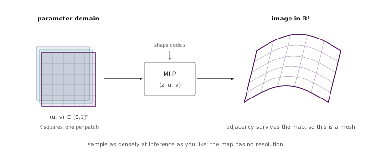
The comparison the lecture draws is between the three explicit decoders side by side on the same input image: a voxel grid, blocky and resolution-limited by the cubic cost of Section 16.8; a point cloud, unstructured and unrenderable; and an AtlasNet surface, smooth and directly usable. The trend across them is toward representations that carry more structure per stored number, and the next step continues it by removing the stored numbers altogether.

16.11 The network is the field

Strip a voxel grid down to what it actually asserts and it is a table of answers to one question: given a point, is it inside the object? Section 16.5 arrived at voxels precisely by precomputing that query on a lattice. The realisation of 2019 was that the precomputation is the mistake. If the question is given a point, what is here, then a network can answer it directly — take coordinates in, give a value out — and the lattice, its cubic cost and its resolution ceiling all disappear at once.

Four papers reached that conclusion within months of each other, differing mainly in what the network outputs. Occupancy Networks and IM-Net predict a binary occupancy, so the surface is the decision boundary of a classifier. DeepSDF predicts the signed distance of Equation 16.8, so the network carries the magnitudes as well as the sign. In every case the model is a function

$$f_\theta : \mathbb{R}^3 \times \mathbb{R}^d \to \mathbb{R}, \qquad (\mathbf{x}, z) \mapsto \text{occupancy or } d(\mathbf{x}), \tag{16.13}$$

conditioned on a latent code $z$ that selects which shape of the learned family is being queried, and the surface of that shape is the level set of Equation 16.4 for the function $f_\theta(\cdot, z)$.

What this buys is the property no discrete representation can have: the model is resolution-free. There is no grid, so there is no maximum detail decided at training time; extracting a mesh at $512^3$ from a network trained on sampled queries costs only more queries, and memory scales with the network’s parameters rather than with the cube of the resolution. NeRF’s own comparison makes the size argument vivid — a competing method that stored a voxel grid per input image needed over $15$ GB for a single scene, where the network weights came to $5$ MB, a factor of roughly three thousand. A network is a very compact way to hold a function that a grid holds badly.

The cost is that every query is a forward pass, and turning the field back into geometry means running marching cubes over a great many of them. It is a representation optimised for asking, which is the containment query of Section 16.4, and it is why implicit methods were positioned exactly right for what came next.

Composition survives the move to networks, too. Local deep implicit functions and their predecessors represent a shape as a collection of small implicit functions with local support rather than one global field, recovering the CSG idea of Equation 16.7 with learned rather than authored primitives, and gaining locality — editing one region no longer perturbs the whole object.

16.12 Geometry and appearance in one function

A deep implicit function trained on occupancy needs occupancy labels, which means 3D supervision, which returns us to Figure 16.5 and the shortage it describes. NeRF makes two changes to Equation 16.13 and between them they remove the requirement entirely.

The first is to widen what the field carries. Instead of one scalar, the network takes a position and a viewing direction and returns a volume density together with a colour:

$$F_\theta : (\mathbf{x}, \mathbf{d}) \mapsto (\sigma, \mathbf{c}), \qquad \mathbf{x} \in \mathbb{R}^3,\ \mathbf{d} \in \mathbb{S}^2 . \tag{16.14}$$

The density $\sigma$ depends on position alone — geometry does not change with where you stand — while the colour may depend on direction, which is what lets the model reproduce specular highlights that move as the camera does. Nothing here is a new kind of object; it is the implicit representation of Section 16.5 extended from geometry to appearance, exactly as Section 16.4 predicted the containment query would demand.

The second change is what makes it trainable. March a ray $\mathbf{r}(t) = \mathbf{o} + t\mathbf{d}$ from the camera through the scene, sample $N$ points along it, and composite them front to back:

$$\hat{C}(\mathbf{r}) = \sum_{i=1}^{N} T_i \, \alpha_i \, \mathbf{c}_i, \qquad \alpha_i = 1 - e^{-\sigma_i \delta_i}, \qquad T_i = \prod_{j=1}^{i-1} (1 - \alpha_j), \tag{16.15}$$

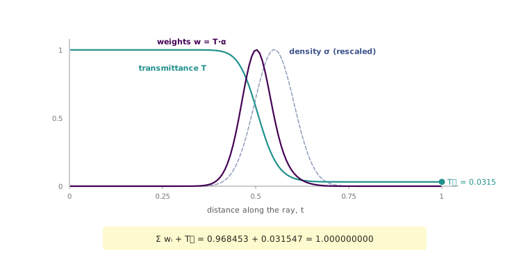
where $\delta_i$ is the distance between consecutive samples, $\alpha_i$ is the opacity that a segment of length $\delta_i$ at density $\sigma_i$ contributes, and $T_i$ is the transmittance — the fraction of light that survives everything nearer the camera. The product of the two, $w_i = T_i \alpha_i$, is how much this sample contributes to the pixel.

This is standard volume rendering from graphics, and the only property NeRF needs from it is that every operation in Equation 16.15 is differentiable with respect to $\sigma_i$ and $\mathbf{c}_i$, which are the network’s outputs. So the loss can be squared error between $\hat{C}$ and the actual pixel of an actual photograph, and gradients flow back through the compositing sum into the field. Training data is a set of images with known camera poses. No 3D ground truth is involved at any point.

The weights have a structure worth naming, because it is what makes the sum behave like a rendering rather than an arbitrary weighted average. Since $T_{i+1} = T_i(1 - \alpha_i)$, each weight is a difference of consecutive transmittances, $w_i = T_i - T_{i+1}$, and summing telescopes:

$$\sum_{i=1}^{N} w_i \;+\; T_{N+1} \;=\; 1 . \tag{16.16}$$

The weights and the light that escapes out the back of the volume partition unity exactly. That is why an opaque surface produces weights concentrated on one sample, why an empty ray produces $T_{N+1} \approx 1$ and a background colour, and why the compositing can never manufacture or lose energy. The generator behind Figure 16.11 evaluates Equation 16.16 on a sampled ray and asserts it to machine precision. It also checks the sum against a closed form, and that check returns something slightly better than convergence: for a slab of constant density the discrete sum equals $1 - e^{-\sigma L}$ exactly, at any number of samples, because the transmittance product telescopes into a single exponential. The discretisation error in Equation 16.15 therefore comes entirely from density varying between samples, which is why NeRF’s hierarchical sampling — spending samples where the weights are large — buys as much as it does.

Figure 16.11: Volume rendering along one ray through a soft-edged surface. Density rises and falls across the surface; transmittance $T_i$ decays monotonically as light is absorbed; the compositing weights $w_i = T_i\alpha_i$ peak before the density does, because transmittance has already begun to fall by the time the density reaches its maximum. That single narrow band of weight is what makes the sum behave like a surface intersection without anyone having to find one. All three curves are evaluated by the generator from the same density profile, and the weights are checked against Equation 16.16.

The consequence reaches beyond reconstruction. The generative pipeline of Section 16.8, which paired a voxel generator with a differentiable projection, can have its voxels replaced by a radiance field — this is what π-GAN and its relatives do — and the resulting model learns 3D-aware image synthesis from photographs alone, with camera viewpoint and object identity as separate controls. Categories no longer need a 3D dataset to be modelled in 3D. That is the payoff Section 16.6 was pointing at.

16.13 Back to explicit, for speed

NeRF’s weakness is visible in Equation 16.15. Producing one pixel requires evaluating a network at every sample along a ray, and the samples are placed along the whole ray because nothing tells the renderer in advance where the object is. Most of them land in empty space and return a density near zero, which is the same waste that Section 16.8 diagnosed in voxel grids, moved from memory into compute. The original method takes on the order of tens of seconds per frame.

3D Gaussian splatting fixes it by changing where the scene is parameterised. NeRF defines its field densely — at every point in space, whether or not anything is there. Gaussian splatting defines it sparsely, storing a set of anisotropic 3D Gaussians, each with a position, a covariance, an opacity and a view-dependent colour, and treating the space between them as empty by definition. This is a point cloud whose points have extent: explicit and non-parametric, back in the top-left cell of Figure 16.4, after the field spent a decade travelling to the opposite corner.

Rendering then becomes projection rather than search. Each Gaussian projects to an ellipse in the image, the ellipses covering a pixel are sorted by depth and alpha-composited with the same Equation 16.15 arithmetic, and no sample is ever spent on a region containing nothing. The representation is optimised by gradient descent through that rasteriser, starting from the sparse point cloud that structure-from-motion already produces during camera calibration, with Gaussians split, cloned and pruned as the fit demands.

Figure 16.12: Two ways to say where the scene is. NeRF queries a network at samples spread along the whole ray, so most evaluations land in empty space; splatting stores primitives only where density is nonzero and projects them, so the empty space costs nothing. This is the same argument that took voxels to octrees in Section 16.8, applied to compute rather than memory.

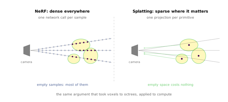
The numbers are the reason the method took over within a year. Against Mip-NeRF360, the strongest quality-oriented radiance-field method at the time, splatting reports higher PSNR — $25.2$ against $24.3$ — while training in $51$ minutes rather than $48$ hours and rendering at $93$ frames per second rather than $0.071$. That last ratio is a factor of about $1{,}300$, and it is the difference between a research artefact and something that runs in a browser. A shorter-trained configuration reaches $135$ frames per second at $23.6$ PSNR, still ahead of the fast baselines it is compared against.

Figure 16.13: Rendering speed against quality, from the numbers 3D Gaussian splatting reports for itself and four baselines; the label on each point is training time. Note the logarithmic speed axis, which spans four orders of magnitude, and that the quality axis does not start at zero — the PSNR differences are real but small next to the speed differences, which is the whole claim.

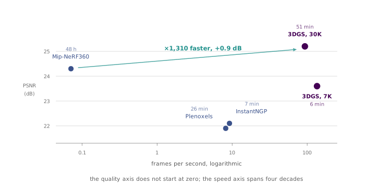
Read against Figure 16.4, the arc is not a march toward implicit representations at all. It is a circuit. Voxels were chosen because a convolution needed a grid; points were chosen because the grid wasted its cells; implicit fields were chosen because the containment query is what rendering asks; and splats were chosen because the field wasted its queries. Each move fixed the previous one’s dominant cost, and the destination happens to sit next to the starting point with a great deal learned in between.

16.14 What geometry leaves out

Every representation so far — points, meshes, fields, splats — describes a shape as an undifferentiated surface. None of them records that a chair’s four legs are copies of one another, that its left and right halves are mirror images, that the seat rests on the base rather than floating near it, or that a bed in a bedroom is against a wall. These regularities are not incidental decoration on the geometry. They are most of what makes an object recognisable as a designed thing, and a generative model that does not represent them has to rediscover them, imperfectly, in every sample it draws.

A structure-aware representation splits a shape into element geometry — the surface of each part, handled by anything in this chapter so far — and element structure, which is what the parts are and how they relate. The design space for the second half is a ladder, and each rung buys a guarantee and costs something.

At the bottom is segmented geometry: an ordinary shape with per-region labels. It is trivial to build from existing models and it guarantees nothing, because a generative model producing labelled geometry must learn to keep its segments coherent and may not. Part sets promote the parts to first-class objects — volumetric primitives or small implicit functions assembled into a whole — which makes each part valid by construction, at the price of saying nothing about how they sit together; nothing stops a leg from floating.

Relationship graphs add edges for adjacency, support and symmetry, so connectivity can be enforced rather than hoped for, but generating graphs is an open problem in a way that generating sequences and trees is not. Hierarchies trade the other way: a tree is much easier to generate, and matches how designed objects decompose — a room contains chairs, a chair has a base, the base has legs — but not every relationship is naturally a tree, and symmetry between siblings is exactly the kind that is not. Hierarchical graphs combine them, keeping a tree for the decomposition and a small graph at each level for the lateral constraints, which is StructureNet’s design and needs a graph network that can encode and decode variable-degree nodes. Its cost is annotation: data in this format is expensive, and PartNet exists largely because it did not otherwise.

At the top are programs. A shape described by the code that constructs it subsumes every other rung, since a program can emit any of them, and it expresses the object’s real degrees of freedom as free parameters — the number of legs, the height of the seat — which is exactly what a parametric representation was for in Section 16.3, now generalised beyond a fixed formula. It is also the hardest format to obtain data in, because almost nothing in the world’s 3D corpora ships with the program that made it.

The ladder is unresolved, and the lecture presents it as such. What it establishes is that the taxonomy of Figure 16.4, which organises the whole of this chapter, is a taxonomy of geometry — and that a full account of a 3D object needs a second axis the chapter has barely touched. Every method in Section 16.7 through Section 16.13 improved how well a surface can be stored, queried and rendered. None of them made a model that knows a chair has four legs because chairs do.

16.15 The map is the result

The first half of this chapter is older than deep learning and reads, at first, like background. It is not. Every architectural decision in the second half is a choice of cell in Figure 16.4, and every one of them was made for a reason stated in Section 16.4: some query got cheap, or some query got expensive.

The reason it is worth carrying the map rather than the list is that the list keeps changing and the map does not. Voxels lost to points because a grid pays $O(n^3)$ for an $O(n^2)$ object. Points lost to parametric decoders because a set has no connectivity and a renderer needs one. Parametric decoders lost to implicit fields because rendering asks what is at this point, which is the one question an explicit representation cannot answer cheaply. Implicit fields lost — for real-time rendering, not everywhere — to splats because answering that question everywhere wastes most of the answers. Four moves, four different dominant costs, and each successor sitting in whichever cell made the current bottleneck disappear.

Two things follow that are worth holding onto past the specific methods. The first is that rendering is the load-bearing bridge, not an output stage. It appears in Section 16.7 as a way to reach ImageNet pretraining, in Section 16.8 as a differentiable projection carrying an adversarial loss, and in Section 16.12 as the entire supervision signal — and each time the underlying reason is Figure 16.5, which shows a 3D data supply that has not caught up and probably will not. A method that can be trained on photographs has access to a corpus that no amount of scanning will match.

The second is that geometry was never the whole problem. Section 16.14 is two minutes of an eighty-minute lecture and it names the thing that none of the preceding representations do: the regularities that make an object a designed object rather than a surface. A splat cloud can reproduce a chair to a fraction of a millimetre and still not encode that it has four legs. Whatever comes after the circuit described here is likely to be judged on that axis rather than on PSNR.