7 CNN Architectures
Lecture 6
Based on Lecture 6 of CS231n, Stanford University, Spring 2025.
7.1 The rest of the kit
A convolutional network is built from six kinds of layer, and Section 6.4 and Section 6.10 have covered two of them while Section 5.1 covered a third. Convolution supplies the learned templates, pooling reduces resolution without learning anything, and the fully connected layer at the end turns whatever the stack produced into class scores. Activation functions were treated in Section 5.3. That leaves two, and both are there for reasons that have nothing to do with representing images.
Normalization layers exist because a deep stack is numerically fragile. The output of one layer is the input to the next, and nothing in the definition of a convolution keeps the scale of its output anywhere near the scale of its input; over thirty layers a modest drift compounds into activations that are either negligible or enormous, and in both regimes the gradient that has to travel back through them is useless. A normalization layer intervenes directly, rescaling its input to a fixed distribution before passing it on. Dropout exists for a different reason entirely: it deliberately damages the network during training, in order that the network cannot come to depend on any particular part of itself.
The two are worth taking together because the second is the first clear instance of a pattern this chapter returns to at length. Dropout is not a mechanism for representing anything. It is randomness injected during training and removed at test time, and the several other techniques that share that shape — data augmentation, and, incidentally, batch normalization — turn out to be doing the same job by the same logic. Section 7.11 makes that argument once, for all of them. Here, dropout is introduced as what it is on the page: a layer.
7.2 Normalization layers
Every normalization layer in current use does the same two things in the same order, and the entire family differs only in a choice made inside the first. Step one computes a mean and a variance from some subset of the activations and uses them to standardize that subset to zero mean and unit variance. Step two undoes this, partially, through two learned parameters — a scale and a shift — applied per feature.
The second step deserves an explanation before the first, because it looks like it cancels the work just done. It does not, and the reason is that the parameters are learned. Forcing every layer’s output to be a unit Gaussian is a strong constraint and not obviously the right one; a layer feeding a sigmoid might want its inputs concentrated near zero, and a layer feeding a ReLU might want a mean well above it. Standardizing and then applying a learned and does not fix the distribution, it fixes the parameterization of the distribution. The mean and variance of the layer’s output are now controlled by two parameters that gradient descent can set directly, instead of emerging as an accident of every weight in every layer below. That the network could in principle recover the identity function by learning and is the point: nothing has been taken away, and something has been made easier to steer.
Take layer normalization, the variant most common today and the one used in essentially every transformer. Given a batch of samples each of dimension , written , the statistics are computed within each sample, across its features:
There are means and variances, one pair per sample. The normalized value and the layer’s output are then
The is a small constant, typically , present only so that a feature vector with no variation does not divide by zero. Note the index on and : they are indexed by feature, not by sample, so there are of each and they are shared across the batch. The statistics vary per sample; the learned correction does not.
Now change the choice. Suppose the statistics are computed per feature instead, averaging over the samples in the batch:
with the variance defined correspondingly. That is batch normalization, and the arithmetic downstream of Equation 7.3 is identical. Only the axis of the average has moved.
For a convolutional network the activations are a four-dimensional block of shape — batch, channel, height, width — and the choice becomes richer, because there are now three axes to average over rather than one. Layer normalization takes one sample and averages over all of its channels and all of its spatial positions: one mean per image. Batch normalization takes one channel and averages over the batch and over space: one mean per channel, computed across every image in the mini-batch. Instance normalization is the intersection, one mean per image per channel. Group normalization splits the channels into a fixed number of groups and normalizes within each, sitting between the layer and instance cases and reducing to each of them at the extremes of the group count.
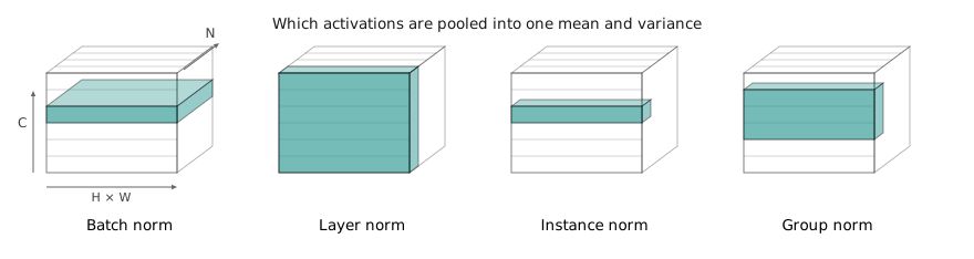
The reason the choice matters — and the reason layer normalization displaced batch normalization in most new architectures — is that batch normalization makes the output for one image depend on the other images that happen to share its mini-batch. During training that is merely strange. At test time it is unusable: predictions must not depend on what else was in the batch, and there may not be a batch at all. Batch normalization therefore has to behave differently in the two regimes. During training it accumulates a running estimate of each channel’s mean and variance across all batches seen, and at test time it uses those fixed estimates in place of the batch statistics. This works, but it introduces a discrepancy between the function being trained and the function being evaluated, it degrades badly when the batch is small enough that its statistics are noisy, and it is a recurring source of bugs in which a model in the wrong mode silently produces different numbers. Layer normalization has none of these problems, because Equation 7.1 never looks outside the sample. It is the same computation at training and at test, for a batch of one thousand or a batch of one.
One caution about the standard explanation. The batch normalization paper attributed the benefit to reducing internal covariate shift, the drift in each layer’s input distribution as the layers below it are updated, and that phrase is still repeated. The empirical case for it is weak: later work found that deliberately injecting distribution shift after a normalization layer does not remove the benefit, and argued instead that normalization helps by making the loss surface smoother, so that the gradient at a point remains a good guide over a larger step. The layer works. The original account of why is not something to repeat with confidence.
7.3 Dropout
Dropout is a layer with no parameters and one hyperparameter. On each forward pass during training it samples a fresh binary mask and multiplies the incoming activations by it, setting each one to zero independently with probability :
A dropped unit contributes nothing forward, and — by exactly the argument of Section 5.10, since multiplication by zero is what a closed ReLU also does — receives no gradient back, so the weights that feed it go unmodified on that step. The mask is resampled every forward pass, so no unit is dropped for long, and is typically in a fully connected layer.
The obvious objection is that this is vandalism. Half the network’s computed features are thrown away at random, training accuracy suffers, and none of it is targeted at anything. The standard defence is that it prevents co-adaptation. Consider a layer near the output of a cat classifier whose units have come to detect ears, a tail, fur, claws. If the training set is such that ears and fur reliably occur together, the layer above can learn a rule that requires both, and that rule will be brittle on any image where one of them is occluded or unusual. Under dropout the two are only sometimes both present, so a rule that requires both is punished during training, and what survives is a broader and more redundant set of correspondences between features and classes. The network is prevented from concentrating its evidence.
A second reading is sharper and explains the test-time behaviour. Each sampled mask defines a different sub-network, and training with dropout trains an enormous ensemble of these sub-networks, all sharing one set of weights. A fully connected layer of units admits masks, a number with more than twelve hundred digits, so no mask is ever seen twice and no sub-network is ever trained to convergence individually. Ensembling normally means averaging the predictions of separately trained models; here the averaging has to be approximated in a single forward pass.
That approximation is the whole of the test-time rule. At test time no units are dropped, which means each unit now receives roughly twice the input it saw during training and every activation downstream is inflated. What is wanted is that the test-time output equal the expected training-time output, and since the expectation of Equation 7.4 is , the fix is to multiply the test-time activations by the keep probability . In practice the scaling is moved to the other side — divide by during training and leave the test path untouched — which is called inverted dropout and is what every framework implements, because it keeps inference free of any dropout-specific arithmetic.
Dropout has largely disappeared from convolutional architectures, and the reason is instructive rather than incidental. It was introduced when the parameter mass of a network sat in large fully connected layers, which is where it does its work; the architectures of Section 7.6 and Section 7.8 moved that mass into convolutions and then removed the large fully connected layers altogether, at which point there was much less left to co-adapt. It survives where those layers survive, in transformers most of all, and in convolutional networks it has been displaced by the regularizers of Section 7.11, which achieve the same end without touching the architecture.
7.4 Activations, settled
Section 5.3 derived what the choice of activation function is a choice between: saturation at both ends for the sigmoid and tanh, a gradient that is exactly zero or exactly one for the ReLU, smoothed variants such as GELU that keep the ReLU’s shape without its kink at the origin. What that section could not supply, because it had no architectures to compare across, is how much the choice is worth.
The answer is: not much, and this is worth stating plainly because the number of proposed activation functions suggests otherwise. The most thorough attempt to find a better one searched a space of candidate functions automatically and reported, for its winner against ReLU on ImageNet with the architecture held fixed, a gain of points of top-1 accuracy on one network and on another. That is the result of an explicit search for the best available replacement; the spread across the functions someone would actually pick between is smaller still. The gap between the architectures compared in Section 7.5 is an order of magnitude larger. An activation function is a decision that should be made once, cheaply and early — ReLU for a convolutional network, GELU where a smooth alternative is conventional, as in transformers — and then left alone while the effort goes somewhere it can pay.
The single exception is the one Section 5.3 already made: do not use a sigmoid or a tanh in the body of a deep network. That is not a matter of a point of accuracy but of whether the gradient survives the trip back at all.
7.5 The revolution of depth
Section 6.12 left the question of how to assemble the layers, and noted that it was settled empirically. The venue for that was the ImageNet challenge, run annually from 2010 to 2017, and its results are unusually legible: one task, one test set, one number per year, over the exact period in which the field changed. What the sequence records is not a series of clever ideas. It is a single variable increasing.
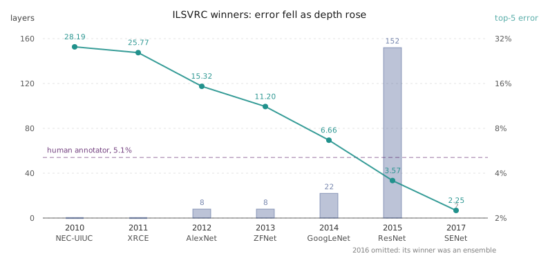
The two entries before 2012 are hand-designed feature pipelines of the kind Section 6.1 described, and their error is around 26%. AlexNet has eight layers and takes it to 15.3%, a margin over the best non-network entry that was itself the news of the year. The 2013 winner has eight layers and refines AlexNet’s hyperparameters. Then 2014, in which two entries arrive at once — VGG with nineteen layers and GoogLeNet with twenty-two — and the error halves again. In 2015 ResNet has a hundred and fifty-two layers and reports 3.57%, passing the 5.1% that careful human annotators achieve on the same thousand categories. The two remaining years refine rather than restructure, and the challenge stopped.
Reading this as a story about depth is not a retrospective imposition; it is what the winning papers say they are doing. But depth alone is not a design, and the interesting content of the period is in the two questions it forced. If more layers are better, what should each layer be — because a network of a hundred and fifty-two distinct hand-chosen layers is not something anybody can design. And why did the answer to the first question stop working at around twenty layers, which it demonstrably did. VGG answers the first. ResNet answers the second.
7.6 VGG: design by rule
VGG is the network that stopped choosing layers individually. Its entire architecture follows from three rules. Every convolution is with stride and padding . Every pooling layer is max pooling with stride . After every pooling layer, the number of channels doubles. Everything else — sixteen or nineteen layers depending on the variant, arranged in blocks of two or three convolutions between pools — is a matter of how many times the rules are applied. AlexNet, by comparison, has filters in its first layer, in its second, thereafter, with strides and pool sizes chosen per layer. VGG looks like a scaled-up AlexNet in a block diagram, and in the respect that matters it is the opposite: it has no per-layer choices left to make.
Each rule earns its place. Consider first why the filters are all , which looks like giving something up — a filter sees almost nothing. Stack three of them and, by the arithmetic of Section 6.8, each output position depends on a window of the input: the first layer’s receptive field is , and each subsequent stride- layer adds one position on each side, so the field grows by two per layer. Three layers and one layer therefore see exactly the same region of the image.
They do not cost the same. For a layer with input and output channels, a convolution holds
weights, while three layers hold
Forty-five per cent fewer parameters for the same receptive field, and the same saving in arithmetic since both are applied at every spatial position. That is the smaller of the two gains. The larger one is that the stack has three nonlinearities where the single layer has one. A convolution, however many channels it has, computes a linear function of its window; the three-layer stack computes a composition of three linear maps separated by ReLUs, which is a strictly larger family of functions over the same window. Smaller filters, stacked, are both cheaper and more expressive. There is no trade here to balance, which is why the rule holds throughout the network rather than at selected layers.
The channel-doubling rule is the one that is easiest to mistake for arbitrary, and it follows from a similar calculation. The cost of a convolutional layer, in both weights and multiplications, is proportional to per output position, and to positions. Halving and at a pooling layer cuts the number of positions by four. Doubling the channels multiplies the per-position cost by four. The product is unchanged:
Every stage of the network therefore performs the same amount of work, and the network spends its arithmetic evenly across scales instead of concentrating it at the resolution it happens to start with. This convention outlived VGG entirely; ResNet uses it, and so does essentially every convolutional architecture since.
What the rules do not do is control where the resources end up, and VGG-16 is the clearest available illustration that the two costs of a network sit in different places.
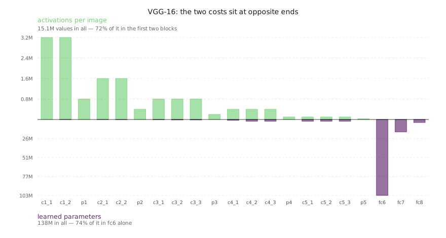
Memory lives at the front. The first convolutional layer produces activations, over three million numbers from a single image, and the first two blocks together account for 72% of the network’s activation memory while holding under a fifth of one per cent of its weights. This is why batch size is limited by early layers and why the input resolution is the most expensive hyperparameter in a convolutional network: both costs scale with .
Parameters live at the back, and specifically in one layer. After the final pooling the activation volume is , and the first fully connected layer maps all of those values to units, which requires
weights — about of VGG-16’s million. One layer, doing nothing structurally interesting, holds three quarters of the model. It is the layer that discards spatial structure by flattening, which Section 6.2 argued against on other grounds, and it is also where dropout was most needed and most effective. Both observations point the same way, and the architecture in the next section acts on them.
7.7 Where depth stopped working
If the VGG rules are right, the obvious experiment is to apply them further. Take a plain convolutional network of twenty layers, build one of fifty-six by the same recipe, train both on CIFAR-10, and compare. The ResNet authors ran it, and the fifty-six-layer network was worse.
The reflex is to call this overfitting: more parameters, less generalization, a familiar story. The reflex is wrong, and the evidence that kills it is in the same figure. The fifty-six-layer network is also worse on the training set. An overfitting model fits the training data too well; this one fits it less well, having strictly more capacity with which to do so. Nothing about generalization is implicated. The deeper network is failing at the easier task.
This is worth stating carefully, because the conclusion is stronger than it first appears. Any function a twenty-layer network computes can be computed by a fifty-six-layer network: take the twenty-layer solution, and set the remaining thirty-six layers to the identity. The deeper network’s hypothesis space contains the shallower one’s entirely, so its optimal training error cannot be higher. The observed training error is higher. Therefore the problem is not representational but optimizational — the solution exists and gradient descent does not find it — and, as the lecture notes, training for longer does not close the gap. The construction just described is what points at the fix. It requires thirty-six layers to learn the identity function, and a stack of convolutions with a ReLU on top has no particularly easy way to do that. Every weight matrix would have to arrive at exactly the right value, and there is no gradient signal pushing any of them there. The identity is available in principle and unreachable in practice.
7.8 Residual networks
The residual block changes what the layers are asked to learn. Where a plain block computes some mapping directly from its input, a residual block computes a correction and adds the input back:
where is the same pair of convolutions a plain block would have contained, and the second addend is the input carried unchanged along a skip connection that goes around them. Rearranged, : the convolutions are no longer fitting the desired output but the difference between the desired output and what already arrived, which is what gives the block its name.
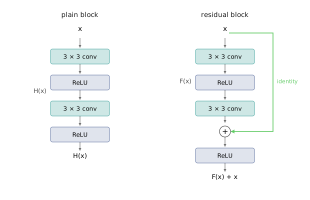
Now reconsider the identity. To make Equation 7.9 compute , the block needs , which it achieves by driving its convolutional weights to zero — a state that weight decay actively pulls towards, that small initialization already starts near, and that gradient descent reaches by shrinking values rather than by coordinating them. The identity has gone from the hardest thing for a block to represent to the easiest. A deep residual network that needs only twenty layers’ worth of computation can switch the rest off, and it can do so smoothly, one block at a time, without any block having to be correct before the others are. Depth stops being a commitment. It becomes a budget the network may decline to spend.
There is a second reading, in terms of gradients rather than functions, that explains why the effect is so reliable. Differentiating Equation 7.9 gives . By the addition rule of Section 5.10, the skip connection distributes the incoming gradient unchanged to both branches, so every block passes its gradient backwards intact regardless of what its convolutions are doing. The gradient reaching layer one of a hundred-and-fifty-two-layer network no longer has to survive a hundred and fifty-one multiplications; there is a path along which it survives none of them. The honest position is that neither reading is a proof — the lecture is explicit that why residual connections work is still argued over — but the empirical fact is not in dispute, and it is why the same connection appears in every transformer.
The full architecture assembles from there with few surprises. A single convolution with stride and a pooling layer reduce the input, a choice the authors report as empirical rather than principled. The body is a stack of residual blocks, each two convolutions, following VGG’s conventions throughout: same padding, same filter size, and periodically a stride- block that halves the spatial dimensions and doubles the channels, which keeps Equation 7.7 satisfied. At a downsampling block the skip connection cannot be a bare copy — the tensors no longer match in shape — so the shortcut carries a convolution with stride to bring into agreement with .
The end of the network is where ResNet departs from VGG most sharply, and Figure 7.3 explains why. There are no large fully connected layers. The final activation volume is reduced to one number per channel by global average pooling — the mean over the entire spatial grid — and a single linear layer maps those channels to the class scores. The hundred-million-parameter layer of Equation 7.8 is gone, and with it most of the network’s parameter count: ResNet-50 has about million parameters against VGG-16’s million, while being three times as deep and considerably more accurate. The deeper variants add one more economy, the bottleneck block, which replaces the two convolutions with a that cuts the channel count by four, a at that reduced width, and a that restores it. The expensive then operates on a quarter of the channels, which is what makes a hundred and fifty-two layers affordable at all.
The family was released at several depths — , , , , — and accuracy improves monotonically with depth across all of them, which is precisely the property Section 7.7 showed plain networks lack. The improvement flattens: the gap from to layers is around a point, and the authors stopped there rather than at a principled limit. What the result established is that depth had not been exhausted in 2014; it had been blocked by an optimization failure, and removing that failure let a decade of architecture work proceed. For roughly five years afterwards, a ResNet was the default backbone for nearly every task in computer vision.
7.9 Initialization
The architecture is now specified, and none of it trains from an arbitrary starting point. Every weight has to be given a value before the first forward pass, and although Section 4.6 treated that as a detail, at depth it is not one.
Two options can be dismissed immediately. All zeros makes every unit in a layer compute the same thing, receive the same gradient, and remain identical forever — the network never breaks symmetry and behaves as though each layer had one unit. All the same nonzero constant fails for the same reason. Whatever is done must be random, and the only remaining question is the scale.
Take a six-layer network of units and draw every weight from a Gaussian with standard deviation , then look at the distribution of activations layer by layer. Layer one produces a reasonable spread. Layer two is narrower. By layer six the activations are indistinguishable from zero. Nothing has gone wrong arithmetically; each layer multiplies by weights smaller than unity in aggregate and the scale shrinks geometrically. The consequence is fatal for training, because a layer whose input is zero produces a zero gradient for its weights — Section 5.10 established that the gradient with respect to a weight is proportional to the activation it multiplies — so nothing below the collapse ever learns. Now raise the standard deviation to . The activations grow instead, layer by layer, and by layer six they are large enough that a tanh saturates completely or a ReLU produces values that overflow into the loss. The gradient dies at the other end.
What the two failures have in common is that the variance of the activations is not preserved from layer to layer, and that suggests the fix. For a linear layer with inputs, weights drawn independently with variance , and inputs independent with variance , each output is a sum of independent products, so
Requiring gives , which is Xavier initialization. It holds the scale of the activations constant however deep the network is, and it is derived rather than tuned: the layer’s own width supplies the number.
Xavier assumes the layer is linear, and a ReLU is not. About half of the outputs of any layer are set to zero, which halves the variance of what the next layer receives, and over many layers a factor of one half per layer is exactly the geometric collapse the derivation was supposed to prevent. He et al. — the same group that produced ResNet — corrected for it by doubling the variance:
This is Kaiming initialization, and it is the default for convolutional networks. For a convolutional layer is the number of inputs to one filter, , not the number of channels. For the six-layer example above it prescribes , between the two values that failed, and the activation histograms hold their shape from the first layer to the last.
It is worth being clear that the whole problem is a symptom rather than a disease, and that normalization layers address the same symptom from the other side. A network with a normalization layer after every convolution is far less sensitive to how it was initialized, because any drift in scale is corrected at the next layer rather than compounding. The two techniques were developed in parallel and both remain in use: initialization gets the first forward pass into a sane range, normalization keeps it there.
7.10 Preprocessing
The same argument applies once more at the input, where the data are not something the network produced and cannot be corrected by a layer that has not run yet. Raw pixels arrive in , all positive and all of comparable magnitude, which is a poor input distribution for the reason Section 7.9 just gave — a layer receiving inputs with a large mean produces outputs dominated by that mean, and the gradients with respect to a row of then all share a sign.
The convention is to center and scale per channel: compute the mean and standard deviation of each of the three colour channels over the training set, then subtract and divide. That is three numbers of each kind, applied identically at every spatial position, which is why the operation costs nothing and is folded into the data loader. Models pretrained on ImageNet ship with the statistics of that dataset baked into their expected input — torchvision’s classification models assume a mean of and a standard deviation of on pixels already scaled to — and applying a different normalization to an image at inference is a common and quiet source of degraded accuracy.
Two points about method rather than arithmetic. The statistics must be computed on the training split alone and then applied unchanged to validation and test data; computing them over the full dataset leaks information about the test set into training, in a small way that is nonetheless indefensible. And the transformation is fixed once and never re-estimated, which is what makes it a property of the model rather than of the batch — the distinction Section 7.2 drew between layer and batch normalization, arriving here for the same reason.
7.11 Noise you add and then average away
Section 7.3 described a layer that behaves differently during training and testing, and the shape of that difference is worth extracting because several unrelated-looking techniques have it. During training, inject randomness into the computation. During testing, remove the randomness and use the average of what it would have produced. The network is being trained not on a fixed function but on a distribution of functions, and asked to do well in expectation, which is why it cannot depend on any accident of one of them.
Dropout is the version that randomizes the network. Data augmentation is the version that randomizes the data, and it is the more important of the two in vision. Rather than train on each image once, apply a random transformation to it every time it is drawn: the label is by assumption unchanged, so the model sees a much larger effective training set and is forced to produce the same answer across the variation the transformation spans. Every augmentation is therefore a claim about which changes to an image do not change what it is, and choosing them is choosing what invariances to demand.
The standard ones are few. Horizontal flips are nearly free and nearly always correct for natural photographs, since a cat facing left is a cat; vertical flips are usually wrong for the same reason, and flips of any kind are wrong for text or digits, where a mirrored is not a . Random cropping and rescaling does the most work: ResNet’s training procedure samples a length uniformly from , resizes the image so its short side is , and takes a random patch, which varies both the scale and the framing of the object on every epoch. Colour jitter perturbs brightness, contrast and saturation, on the claim that the identity of an object does not depend on the lighting it was photographed under. Cutout zeroes a random rectangle of the image outright, forcing the classifier to work from partial evidence rather than one decisive region — the same argument dropout makes about features, transposed to pixels. It helps substantially on small datasets like CIFAR-10 and much less on ImageNet, which is the general pattern for regularization: the less data there is, the more of it is worth adding.
The test-time half of the pattern is usually just “do nothing”, since the identity transformation is the natural centre of the distribution. It need not be. ResNet’s reported ImageNet numbers use test-time augmentation, evaluating each image at five scales with ten crops each — four corners, the centre, and horizontal flips of all five — and averaging the fifty sets of scores. That is the averaging step performed explicitly rather than approximated, and it buys a fraction of a point for fifty times the inference cost, which is why it appears in competition results and almost nowhere else.
Batch normalization belongs to this family too, and it is a nice check on whether the pattern has been understood. Its training-time output depends on which other images share the batch, which is a source of randomness; its test-time output uses running averages accumulated over training, which is the averaging step. That is precisely the dropout structure, arrived at accidentally by a technique designed for something else entirely — and it explains the observation, otherwise puzzling, that a network with batch normalization often needs less explicit regularization than one without.
The practical reading of all this is a dial rather than a checklist. Add regularization when the training accuracy is far above the validation accuracy, remove it when the two are equal and both are low, and choose the specific mechanism by what invariance the problem actually has. Section 7.13 is where that judgement gets made.
7.12 Transfer learning
Everything so far has assumed a million labelled images. Almost no real problem has one, and the reason convolutional networks are nonetheless usable on problems with a few thousand examples is the observation Section 6.6 began: the features a network learns are far less specific to its training task than the task would suggest. AlexNet’s first layer, trained to separate a thousand categories of photograph, contains oriented edges and colour-contrast patches — structures that are useful for any problem involving natural images and were not chosen for ImageNet. The same holds, less obviously, several layers up. Take the activations of the penultimate layer of a trained network as a feature vector and find nearest neighbours in that space, and images land near each other when they depict similar things, including things the network was never trained to name.
The procedure that follows is short. Train a network on a large dataset — or download one, since the pretrained weights for every standard architecture are a line of code away. Discard the final classification layer, which is the only part specific to the original label set. Replace it with a fresh layer of the right output size for the new problem, and train.
What varies is how much of the rest is allowed to move, and the answer depends on two things: how much data the new problem has, and how much it resembles the old one. With very little data and a similar domain, freeze everything and train only the new final layer. The pretrained network is then a fixed feature extractor and the trainable model is a linear classifier on its output — cheap, fast, and hard to overfit, since there are few parameters to overfit with. This is the setting in which DeCAF and related work found that features from a network trained on ImageNet, with a linear classifier on top, beat purpose-built systems on tasks the network had never seen. With a similar domain and a substantial dataset, initialize from the pretrained weights and fine-tune the whole network at a learning rate perhaps a tenth of what would be used from scratch — small enough that the existing features are refined rather than destroyed in the first few steps, while the freshly initialized final layer produces large gradients.
The remaining two cases are less tidy. A large dataset in a different domain — medical scans, satellite imagery, microscopy — can be fine-tuned end to end or trained from scratch, and which wins is an empirical question with no reliable prior. A small dataset in a different domain is the genuinely hard case: there is not enough data to train and not enough similarity for the transfer to carry, and the useful move is to find a pretrained model closer to the target domain rather than to accept ImageNet and hope. There is no technique here that always works.
Between freezing the last layer and fine-tuning everything lies a continuum, and much of the interesting recent work is in it. Unfreezing the last few blocks is the obvious intermediate. More sophisticated is LoRA, which fine-tunes every layer but constrains the update to each weight matrix to be low-rank, so that a small number of new parameters expresses a change to a large number of old ones — structurally the trick of Equation 7.9 applied to weights instead of activations, learning the difference from the pretrained model rather than the model.
The framing worth taking away is not that transfer learning is a workaround for insufficient data. Pretraining on a large corpus and adapting to the task at hand is the default way models are built now, in vision and elsewhere; training a network from random initialization on a task-specific dataset is the special case, reserved for when the dataset is enormous or genuinely unlike anything already trained on.
7.13 Choosing hyperparameters
The architecture, the initialization, the regularizers, the learning rate and its schedule from Section 4.11 — all of it has to be set, and there are more free choices here than a search can cover. What makes it tractable is an order, in which the cheap diagnostics run first and each step assumes the previous one passed.
Check the initial loss before anything else. A softmax classifier over classes at initialization should produce roughly uniform scores, and therefore a loss of — about for CIFAR-10 and for ImageNet. Disable regularization and run one forward pass. If the number is not close, something is wrong in a way no amount of tuning will fix, and the second before it takes to check is the cheapest debugging in deep learning.
Then overfit a tiny sample. Take a handful of training examples — a dozen, or even one — turn off all regularization, and train until the loss reaches zero. A model that cannot memorize twelve images cannot learn a million, and failure here is nearly always a bug rather than a hyperparameter: a mismatch between predictions and labels, a detached gradient, a learning rate off by orders of magnitude. This is the standard first move when training does not work, and it also gives a rough sense of which learning rates move the loss at all.
With that passing, find a learning rate on the full training set. Turn on a small weight decay and try the usual ladder — down to — asking only which value drops the loss substantially within about a hundred iterations. This is not a search for the best learning rate but for the right order of magnitude, and it is fast because it does not require training to completion.
Only now is a search worth running: a coarse grid over the few hyperparameters that matter, each configuration trained for one to five epochs, then a refined range around whatever region looked best, trained longer. And when the search covers more than one dimension, sample the configurations randomly within their ranges rather than laying them out on a grid. The argument, from Bergstra and Bengio, is that the hyperparameters are almost never equally important. A grid of nine points over two parameters tries only three distinct values of each, so if one of them barely matters, six of the nine runs are re-measuring the same three values of the one that does. Nine random points try nine distinct values of every parameter. The advantage grows with the number of dimensions and with how unequal the importances are, which in practice is very.
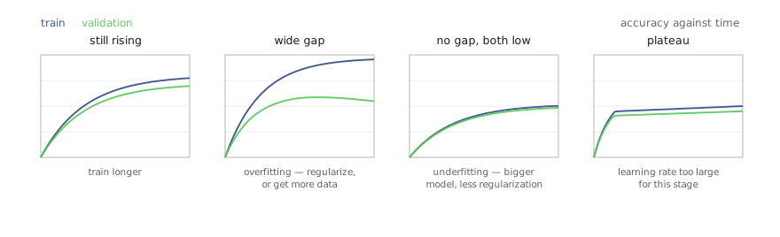
The last step of the loop is to look at the curves, and the information is almost entirely in the gap between them. Both still rising means the run was stopped too early: train longer before concluding anything. A large and widening gap, with training accuracy climbing while validation accuracy flattens or falls, is overfitting, and the response is more regularization or more data — the dial of Section 7.11. No gap at all, with both curves low, is underfitting, and calls for the opposite: less regularization, a longer run, or a larger model. A loss that falls sharply and then plateaus at a poor value usually means the learning rate is too large for the current stage, which is what the schedules of Section 4.11 exist to address. Then return to the search with what was learned, and repeat.
7.14 What this leaves
Two chapters ago there was an operator. There is now a network that can be specified end to end and trained to a competitive result, and it is worth noticing how little of what this chapter added is about images. The convolution encodes something true about pictures. Normalization, dropout, careful initialization, augmentation, transfer learning, and the hyperparameter protocol encode nothing of the sort: they are what it takes to optimize a deep composition of functions, and they transfer to architectures that have no convolutions in them at all. The residual connection of Equation 7.9 and the layer normalization of Equation 7.2 are in every transformer, unchanged.
What the architectures established is narrower and more specific. VGG showed that a network can be specified by a rule rather than designed layer by layer, and that small filters stacked deep beat large filters used shallowly. ResNet showed that the limit on depth encountered in 2014 was a failure of optimization rather than of representation, and removed it. Neither result says anything about what the convolution should be, and both are about how to build with it — which is why the second one survived the convolution’s decline. When the field moved to attention, it kept the skip connections.
The gap that remains is the one Section 7.6 opened and did not close: the classifier at the end of a convolutional network produces one label for a whole image, and almost nothing anyone wants from computer vision has that form. Where in the frame is the object, how many are there, which pixels belong to it, and what happens when the answer must be a sequence rather than a class. Those questions need a different output structure, and in some cases a different architecture entirely.
References
- J. L. Ba, J. R. Kiros and G. E. Hinton, “Layer Normalization,” 2016. arXiv:1607.06450
- J. Bergstra and Y. Bengio, “Random Search for Hyper-Parameter Optimization,” JMLR 13:281–305, 2012. Paper
- T. DeVries and G. W. Taylor, “Improved Regularization of Convolutional Neural Networks with Cutout,” 2017. arXiv:1708.04552
- J. Donahue et al., “DeCAF: A Deep Convolutional Activation Feature for Generic Visual Recognition,” ICML, 2014. arXiv:1310.1531
- X. Glorot and Y. Bengio, “Understanding the Difficulty of Training Deep Feedforward Neural Networks,” AISTATS, 2010. Paper
- K. He, X. Zhang, S. Ren and J. Sun, “Delving Deep into Rectifiers: Surpassing Human-Level Performance on ImageNet Classification,” ICCV, 2015. arXiv:1502.01852
- K. He, X. Zhang, S. Ren and J. Sun, “Deep Residual Learning for Image Recognition,” CVPR, 2016. arXiv:1512.03385
- J. Hu, L. Shen and G. Sun, “Squeeze-and-Excitation Networks,” CVPR, 2018. arXiv:1709.01507
- S. Ioffe and C. Szegedy, “Batch Normalization: Accelerating Deep Network Training by Reducing Internal Covariate Shift,” ICML, 2015. arXiv:1502.03167
- A. Krizhevsky, I. Sutskever and G. E. Hinton, “ImageNet Classification with Deep Convolutional Neural Networks,” NeurIPS, 2012. Paper
- P. Ramachandran, B. Zoph and Q. V. Le, “Searching for Activation Functions,” 2017. arXiv:1710.05941
- A. S. Razavian et al., “CNN Features Off-the-Shelf: An Astounding Baseline for Recognition,” CVPR Workshops, 2014. arXiv:1403.6382
- O. Russakovsky et al., “ImageNet Large Scale Visual Recognition Challenge,” IJCV 115:211–252, 2015. arXiv:1409.0575
- S. Santurkar, D. Tsipras, A. Ilyas and A. Madry, “How Does Batch Normalization Help Optimization?,” NeurIPS, 2018. arXiv:1805.11604
- K. Simonyan and A. Zisserman, “Very Deep Convolutional Networks for Large-Scale Image Recognition,” ICLR, 2015. arXiv:1409.1556
- N. Srivastava et al., “Dropout: A Simple Way to Prevent Neural Networks from Overfitting,” JMLR 15:1929–1958, 2014. Paper
- C. Szegedy et al., “Going Deeper with Convolutions,” CVPR, 2015. arXiv:1409.4842
- Y. Wu and K. He, “Group Normalization,” ECCV, 2018. arXiv:1803.08494