6  Convolutional Networks

Lecture 5

Based on Lecture 5 of CS231n, Stanford University, Spring 2025.

6.1 Two places to put the design

For about a decade before any of this worked, the field solved image classification with a pipeline that had a learned classifier at the end of it and something else in front. That something else was a feature extractor: a function, written by a person, that converted the pixels of an image into a vector believed to capture what mattered about it. The linear classifier of Section 3.4 was then fitted not to the pixels but to that vector. Understanding what the convolution is for is easier from this starting point than from a blank page, because the convolution is not the first attempt to give a classifier something better than raw pixels — it is the attempt that stopped choosing.

The simplest of these representations is a colour histogram. Divide the space of colours into some fixed set of buckets, assign every pixel of the image to the bucket its colour falls in, and let the feature vector be the count of pixels per bucket. The resulting representation is entirely insensitive to where anything is: an image with a red patch in the top-left corner and the same image with the patch moved to the bottom-right produce identical histograms, while in pixel space they have almost nothing in common. That is either exactly what you want, if you are sorting ripe apples from unripe ones, or a catastrophe, if you are not.

The histogram of oriented gradients (HoG) is the dual of that trade. It discards colour and keeps geometry. The image is divided into eight-by-eight pixel cells; within each cell the local edge directions are quantised into nine orientation bins and counted; the counts are concatenated. A $320 \times 240$ image yields a $40 \times 30$ grid of cells and therefore $30 \times 40 \times 9 = 10{,}800$ numbers. What survives is the pattern of oriented structure across the image — the diagonal veins of a leaf, the circular outline of an eye — with the colours thrown away.

A third family borrowed its idea from document retrieval. Bag-of-words representations first build a codebook: extract patches at random from a corpus of images, cluster them, and call the cluster centres visual words. An image is then encoded by matching each of its patches to the nearest word and counting how often each word occurs, exactly as a document is encoded by the frequencies of the terms in it. The version of this used for scene classification treats an image as an unordered collection of local appearances, which is a strong assumption and, for a while, a productive one.

Asked which of these representations was best, practitioners generally answered by using all of them: extract several, concatenate the results, and hand the classifier a long vector assembled from many partial views of the image. It is not an elegant answer, and its inelegance is a symptom.

Set the two systems side by side. Both take the pixels of an image and emit ten class scores. In the first, a fixed function computes features and a learned linear classifier sits on top; in the second, the whole path from pixels to scores is differentiable and every parameter in it moves under gradient descent. The systems differ only in where the boundary falls between what a person specified and what the data determined. Pushing that boundary all the way back to the pixels is the entire content of the phrase end-to-end learning, and the argument for doing so is not that human intuition is worthless but that it is a bottleneck: a person may be wrong about which aspects of the problem matter, and even when right, may be unable to write down the function that extracts them.

It would be a mistake to read this as the abolition of design. The convolutional network is not what you get by removing the human from the pipeline; it is what you get by moving the human’s contribution one level up. A feature extractor is a particular function. An architecture is a family of functions — specified by which operators appear in the computational graph, in what order, with what tensor shapes — inside which gradient descent selects a member. Choosing the family remains a design act, and a consequential one; the next several chapters are largely about how that choice has been made and remade. What has changed is that the design is now expressed in a language the optimizer can work inside of.

6.2 What flattening throws away

The only architecture available so far is the one from Section 5.1: reshape the image into a vector, multiply by a matrix, apply a ReLU, repeat. Applied to CIFAR-10, the $3 \times 32 \times 32$ input becomes 3072 numbers and the first weight matrix is $100 \times 3072$. The reshape looks like bookkeeping. It is not.

Consider what the model would do if the pixels were shuffled. Fix any permutation of the 3072 input positions, apply it to every training and test image, and permute the columns of $W_1$ to match. The two networks compute identical outputs on identical inputs, reach identical losses, and generalise identically. A fully connected network cannot distinguish a photograph from a scrambled version of the same photograph, provided the scrambling is the same every time. Whatever information is carried by the fact that pixel 33 sits directly beneath pixel 1 is information the architecture has no way to use.

Figure 6.1: Left: a $4 \times 4$ image, with one pixel and its four neighbours marked. Right: the same pixels after flattening. Two of the four neighbours land beside the pixel; the other two land a full row away, at distance 4, and would land at distance 224 in a real image. The layer that reads this vector treats all 16 positions as unrelated coordinates, so any consistent re-shuffling of them gives an identical model. Drawn for these notes.

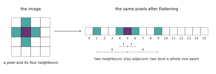
The second cost is arithmetic. As Section 5.2 described, a row of $W_1$ is a template compared against the whole image by a 3072-dimensional dot product, and the comparison is anchored: the template’s entry for position 500 is only ever multiplied against the pixel at position 500. A row that has learned to respond to a wheel in the lower-left of the frame contributes nothing when the wheel appears in the upper-right, and a second row must learn the same pattern again from scratch for the new location. The parameter count grows with the area of the image multiplied by the number of patterns, and the training data must exhibit every pattern in every place.

Both problems point at the same two facts about images, neither of which the fully connected layer knows. The first is locality: what a pixel means is largely determined by the pixels near it, so a feature worth computing can usually be computed from a small neighbourhood. The second is translation: a pattern signifies the same thing wherever it occurs, so whatever computation is applied at one location should be applied unchanged at every other. An operator that assumes both is not a heuristic bolted onto a general architecture. It is a narrower hypothesis class chosen because the narrowing is true.

6.3 A bit of history

Convolutional networks are old enough that their arrival can be dated twice. The architecture used for handwritten digit recognition in LeCun et al. (1998) — a body of alternating convolution and downsampling layers, feeding a small stack of fully connected layers, the whole thing trained by backpropagation — is recognisably the same object as the networks of the mid-2010s. It worked. It was also expensive, on hardware without anything resembling a GPU, and the datasets that would have rewarded a larger version of it did not yet exist.

Both constraints lifted at once. AlexNet, in 2012, is structurally the 1998 network with more layers, wider layers, a training set of a million labelled images and a pair of GPUs to train on, and Section 2.9 describes what it did to the ImageNet leaderboard. For roughly the following eight years, the answer to almost any question about images was a convolutional network: object detection, semantic segmentation, image captioning, and — in the form of the U-Net that denoises the latent in latent diffusion models — the first text-to-image systems that worked well enough to be worth arguing about. When this course was first taught in 2015 it was called Convolutional Neural Networks for Visual Recognition, which was a reasonable name at the time because the two halves of it referred to nearly the same thing.

The name changed because the field did. The transformer was published in 2017 for machine translation and spent a few years confined to text, until the Vision Transformer, presented at ICLR in 2021, cut an image into patches, treated the patches as a sequence of tokens, and ran essentially the unmodified language architecture over them. Across many of the tasks listed above it turned out that replacing the convolutional network with a transformer and changing nothing else improved results, and that the improvement widened as data and compute were scaled up.

That is an honest reason to be careful about how hard convolution is sold, and not a reason to skip it. Convolutional networks remain in wide practical use, particularly where inputs are small or latency is tight; large modern systems are frequently hybrids, with convolutional stems, convolutional decoders, or convolutional blocks interleaved with attention. The more durable reason to study the convolution first is that it is the clearest case in the subject of a prior about the data being written directly into an operator, and of what that buys — which is a lens that applies just as well to the architectures that displaced it.

6.4 The convolution layer

The generalisation from a fully connected layer to a convolutional one is smaller than it looks, and the right way to see it is through the dot product. A dot product between two vectors is large when they point in the same direction and zero when they are orthogonal, so any layer built out of dot products is performing template matching. The fully connected layer holds ten templates, each the size of the entire input, and reports how well each one matches the whole image. Keep the templates and the matching; change only the size of the templates.

A convolutional layer therefore does not flatten its input. It receives the image as the three-dimensional tensor it is, $3 \times 32 \times 32$, with two spatial dimensions and a channel dimension of depth 3 for the colours. Its templates, called filters or kernels, are small along the spatial dimensions and full-depth along the channels: a $3 \times 5 \times 5$ filter is a five-by-five patch of learnable weights on each of the three input channels. Filters always extend the full depth of the input volume, so there is only one spatial size to choose.

Position that filter over one $3 \times 5 \times 5$ chunk of the image, take the dot product of the filter with the chunk — a dot product in $5 \cdot 5 \cdot 3 = 75$ dimensions — and add a scalar bias. The result is a single number reporting how strongly this piece of the image resembles the template. Now slide the filter to every spatial position and repeat. A $5 \times 5$ filter fits into a $32 \times 32$ image in 28 positions horizontally and 28 vertically, so the numbers arrange themselves into a $28 \times 28$ grid, which is called an activation map. The map is an image of the filter’s agreement with the input, evaluated everywhere.

Figure 6.2: One filter, applied. The filter spans all three input channels and five pixels in each spatial direction, so each placement contributes a 75-dimensional dot product plus a bias, producing one scalar. Sliding it over the 28 by 28 valid placements fills an activation map. Six filters produce six such maps, stacked into a $6 \times 28 \times 28$ output volume whose channel dimension indexes filters rather than colours. Drawn for these notes.

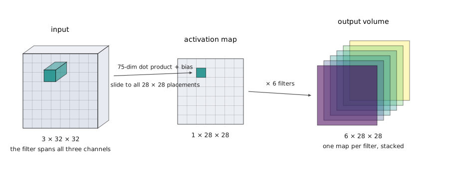
One filter answers one question about every location. A layer asks several. Six filters of shape $3 \times 5 \times 5$ — a single parameter tensor of shape $6 \times 3 \times 5 \times 5$, accompanied by a bias vector with one entry per filter — are each slid across the input independently, and the six resulting maps are stacked along a new channel dimension to give an output of shape $6 \times 28 \times 28$. Nothing couples the filters to each other; the layer is six separate slidings whose results are stored in one tensor.

That output tensor supports two readings, and both are worth carrying. Read by channel, it is six activation maps, each showing where in the image one particular template fired. Read by position, it is a $28 \times 28$ grid at each point of which sits a six-dimensional vector describing the local appearance of the image there. The second reading explains why the output is legitimately an input for another convolution: it is again a stack of spatial planes, differing from the original image only in having six channels of learned features instead of three channels of colour.

In practice the layer is applied to a batch. With $N$ images at once, an input of shape $N \times C_\text{in} \times H \times W$ meets a filter tensor of shape $C_\text{out} \times C_\text{in} \times K_h \times K_w$ and a bias of length $C_\text{out}$, and produces

$$N \times C_\text{out} \times H' \times W', \tag{6.1}$$

where $H'$ and $W'$ are the numbers of valid filter placements, computed in Section 6.7. Four indices is the working dimensionality of nearly everything that follows.

One point deserves emphasis because it is easy to lose among the shapes. Nobody writes the filters. They are initialised randomly and learned by gradient descent, exactly as the weight matrices of Section 5.1 are, and the gradient of the loss with respect to each scalar in each filter is obtained by the backward traversal of Section 5.8 with no new machinery — the layer supplies a forward rule and a local derivative, which is all the interface of Section 5.11 requires of it. What a person chooses is the number of filters and their spatial size — hyperparameters, fixed before training begins because they fix the shapes of the tensors, and tuned by cross-validation like the hyperparameters of Section 3.3. What the data chooses is every number inside them.

6.5 Stacking convolutions

A convolutional network is a computational graph in which some of the nodes are convolutions. A first layer might apply six $3 \times 5 \times 5$ filters to a $3 \times 32 \times 32$ image and produce $6 \times 28 \times 28$; a second might apply ten $6 \times 5 \times 5$ filters to that and produce $10 \times 24 \times 24$; and so on, the input depth of each layer fixed by the output depth of the one before it. Because the layer is just another node with a forward rule and a local derivative, it slots into the graph beside the fully connected layers and losses already defined, and the whole network is trained by the same loop: batch, forward, loss, backward, step.

Stacking convolutions directly on top of one another, however, gains nothing. The argument is the one from Section 5.2 in different clothing. A convolution is a linear function of its input, so the composition of two convolutions is linear, and in fact is itself a convolution — two stacked $5 \times 5$ layers compute some $9 \times 9$ convolution, which a single layer with $9 \times 9$ filters could have computed directly. Depth without a non-linearity buys a larger filter and nothing else. So a ReLU is applied elementwise to every activation map after every convolution, and it is the interleaving, not the stacking, that makes depth mean anything.

The layer’s hyperparameters are few, and worth separating from its parameters once and for all. The number of output channels $C_\text{out}$ and the kernel size $K$ set the shape of the weight tensor and are chosen before training; the stride and padding of Section 6.7 join them. The weights and biases inside that tensor are parameters, initialised randomly and moved by the optimizer. It is a distinction the shapes make obvious — a hyperparameter is something a gradient cannot be taken with respect to, because changing it changes what the tensors are.

Filters within one layer conventionally share a spatial size, which is a decision about implementation rather than about modelling: a fixed kernel size makes the layer a single dense arithmetic kernel that a GPU can execute efficiently. Architectures that want several receptive field sizes at one depth get them by running several convolutional layers in parallel and concatenating the results — the Inception module of the next chapter is exactly this — which keeps the primitive simple and pushes the variety into the graph built from it.

6.6 What the filters learn

Three architectures, three answers to the question of what a learned weight looks like. A linear classifier holds one template per class, each the size of the whole image, and Section 3.4 showed what those templates look like when visualised: blurry class averages, with the two-headed horse as the emblem of their limits. A fully connected hidden layer holds a bank of such whole-image templates, no longer tied one-to-one to classes but still each spanning the entire frame. A convolutional layer holds a bank of local templates, each far too small to cover the image and each applied at every position in it.

Because a first-layer filter has exactly three channels and a small spatial extent, it can be displayed as what it is: a tiny colour image. AlexNet’s first layer is 64 filters of shape $3 \times 11 \times 11$, and rendering them as sixty-four eleven-pixel thumbnails shows two recurring kinds. Some are oriented edges — a light half against a dark half, the boundary running vertically, horizontally or at an angle, at a range of spatial frequencies. The rest are opposing-colour patches: green against red, pink against green, responding to colour contrast with little spatial structure. Nothing in the training objective asked for either. The network was told to classify a thousand categories of photograph and these are what minimising that loss produced.

The result is close to universal. Convolutional networks trained on different datasets, for different tasks, with different architectures, converge to first layers that look substantially like this one. It is also a rediscovery: the oriented-edge detector is precisely what Section 2.3 describes Hubel and Wiesel finding in the cat’s primary visual cortex in 1959, arrived at here by gradient descent on labelled photographs rather than by evolution. That two such different processes settle on the same first operation is a reasonable hint that the operation is forced by the statistics of natural images rather than by either process.

Figure 6.3: Sixty-four templates at eleven pixels square, on the same value ramp. The first six rows are Gabor functions — an oriented sinusoid under a Gaussian envelope — at eight orientations, three spatial frequencies and two phases; the last two rows are centre-surround blobs at four scales and both polarities. These are not filters from a trained network. They are the analytic family that trained first layers reliably approximate, drawn here because the widely reproduced grid of AlexNet’s real first layer is a figure from that paper and cannot be used in these notes. The point they carry is the one that matters: a template this small can encode an edge at an orientation and a scale, or a blob against its surround, and very little else. Computed for these notes.

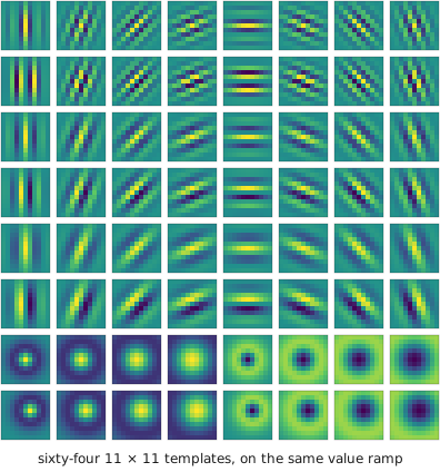
That the filters within a layer end up different from one another is not automatic, and the reason is worth pausing on. Suppose every filter in a layer were initialised to the same values. Each would then compute the same activation map, receive the same upstream gradient, and take the same step, forever; the layer would be a single filter copied $C_\text{out}$ times, with $C_\text{out}$ times the cost and none of the benefit. Random initialisation, with a different draw per filter, is what breaks this symmetry, and the diversity visible in a trained first layer is diversity that the initialisation made possible and the loss then found a use for.

Deeper layers cannot be shown this way. A filter in the sixth convolutional layer might have shape $512 \times 3 \times 3$, which is not an image of anything; its input is a stack of learned features, not colours, so displaying its weights as a picture is meaningless. The standard substitute is to run a large set of images through the network, find the input patches that drive a given filter hardest, and look at those. Done for a sixth layer of an ImageNet model, the resulting patches group into recognisable things: one filter answers to eyes, another to fragments of text, another to wheels and the upper arcs of circles. The progression from edges to parts is not designed and not supervised. It is what happens when each layer is given the previous layer’s features to build from.

6.7 Padding, stride, and the shape arithmetic

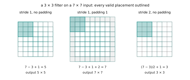
The output size in Equation 6.1 was deferred; it is elementary, and the two hyperparameters that appear in it are both introduced to fix problems it creates. Ignore the channel dimension, which never affects spatial size, and consider a $7 \times 7$ input with a $3 \times 3$ filter. The filter can be placed with its left edge at column 1, 2, 3, 4 or 5 and nowhere else, so the output is $5 \times 5$. In general an input of extent $W$ and a filter of extent $K$ admit

$$W' = W - K + 1 \tag{6.2}$$

placements along each axis. Every convolution therefore shrinks its input, and the shrinkage compounds: seven successive $5 \times 5$ layers reduce a $32 \times 32$ map to $4 \times 4$, and an eighth cannot be applied at all. Some architectures live with this. Most would rather not have the depth of the network limited by an accident of arithmetic, and rather not recompute every shape each time a layer is inserted.

The fix is to pad the input with $P$ rows and columns of zeros on every side before sliding the filter, which restores the placements lost at the border:

$$W' = W - K + 1 + 2P. \tag{6.3}$$

Setting $P = (K-1)/2$ makes $W' = W$, so the map keeps its spatial size through the layer. This is called same padding and is the usual choice; it also explains why kernel sizes are almost always odd, since $(K-1)/2$ is an integer only then. A $3 \times 3$ convolution is paired with $P = 1$, a $5 \times 5$ with $P = 2$, and the spatial dimensions become something the architect sets deliberately rather than something that erodes.

Downsampling, when wanted, is then requested rather than suffered. A strided convolution moves the filter $S$ positions at a time instead of one, so a $3 \times 3$ filter with stride 2 on a $7 \times 7$ input lands in three places along each axis and returns $3 \times 3$. Combining all three:

$$W' = \frac{W - K + 2P}{S} + 1. \tag{6.4}$$

Figure 6.4: Left: a $3 \times 3$ filter on a $7 \times 7$ input at stride 1, giving five placements per axis and a $5 \times 5$ output. Centre: one ring of zero padding restores the lost border placements, and the output is $7 \times 7$ again. Right: stride 2 on the unpadded input takes every other placement, giving $3 \times 3$. All three are Equation 6.4 with different arguments. Drawn for these notes.

A stride that does not divide $W - K + 2P$ leaves the division inexact, and implementations resolve it by taking the floor — the trailing rows and columns that no placement reaches are simply not looked at. It is a small thing and a common source of off-by-one confusion when a network is being assembled from shapes.

6.8 Receptive fields

Every element of a convolution’s output is a dot product over a $K \times K$ window of the input, so it depends on exactly $K^2$ input positions and is blind to the rest of the image. That window is the element’s receptive field. Composing layers widens it: a $3 \times 3$ filter in the second layer reads nine adjacent first-layer outputs, each of which read a $3 \times 3$ window, and those windows together span $5 \times 5$ of the original image. Each further layer adds $K - 1$, so after $L$ convolutions of kernel size $K$ the receptive field in the input is

$$1 + L(K - 1) \tag{6.5}$$

pixels across. The phrase is used in two senses that are easy to confuse and worth keeping apart: the receptive field of a unit in the previous layer is always $K \times K$, while its receptive field in the input image is what Equation 6.5 describes.

Figure 6.5: Three stacked $3 \times 3$ convolutions, drawn in one spatial dimension so the dependencies are visible. One output element reads three elements of layer 2, which between them read five of layer 1, which between them read seven of the input — $1 + 3 \times 2 = 7$, as Equation 6.5 gives. The growth is two pixels per layer regardless of how deep the stack becomes. Drawn for these notes.

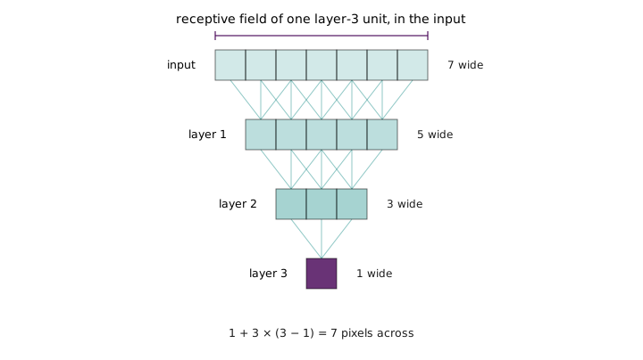
Linear growth is the problem. With $K = 3$ the receptive field widens by two pixels per layer, so an output unit that must see all of a $224 \times 224$ image requires 112 convolutional layers to do it, and a $1024$-pixel image requires more than 500. Classifying an image means combining evidence from all of it, and a network whose deepest units still see only a fraction of the frame cannot do that at any reasonable depth. This is also the answer to why deeper filters respond to larger structures: a unit can only be selective for an eye once its receptive field is big enough to contain one.

The remedy is to shrink the image inside the network rather than to lengthen the network. If a layer downsamples by a factor of two, every subsequent convolution’s receptive field, measured back in the original image, is worth twice as much — the field grows geometrically with depth instead of arithmetically, and a few dozen layers suffice for any image size that will be met in practice. Strided convolution is one way to do it. Pooling, in Section 6.10, is the other.

6.9 Counting a layer

Everything above is arithmetic, and the arithmetic is worth doing once on a concrete layer, because the three numbers it produces — output shape, parameter count, operation count — are what an architecture is judged by. Take a $3 \times 32 \times 32$ input and a layer of ten $5 \times 5$ filters with stride 1 and padding 2.

The output shape follows from Equation 6.4: $(32 - 5 + 2 \cdot 2)/1 + 1 = 32$ along each spatial axis, and ten filters give ten channels, so the layer emits $10 \times 32 \times 32$. The parameter count follows from the filter shape: each filter is $3 \times 5 \times 5 = 75$ weights plus one bias, so 76 parameters, and ten filters give 760. The operation count follows from the output shape and the filter size together: there are $10 \cdot 32 \cdot 32 = 10{,}240$ output elements, each a 75-dimensional dot product, so $75 \cdot 10{,}240 = 768{,}000$ multiply-adds.

Set that against a fully connected layer doing nominally the same job — 3072 inputs to 10,240 outputs. It would hold about $31.5$ million weights and perform about $31.5$ million multiply-adds. The convolution reaches the same output size with roughly one forty-thousandth of the parameters and one fortieth of the arithmetic. The parameter saving comes from weight sharing, since one filter serves all 1024 positions instead of each position owning its own weights; the arithmetic saving comes from locality, since each output consults 75 inputs instead of 3072. These are the two priors of Section 6.2, and this is their price in cash.

The asymmetry between the two counts matters more than either. Doubling the height and width of the input leaves the parameter count of a convolutional layer completely unchanged and quadruples its arithmetic. A convolutional network’s size is a property of its architecture; its cost is a property of what you feed it. Nothing similar is true of a fully connected layer, whose weight matrix must grow with the input.

The full contract of the layer, then. It takes $C_\text{in} \times H \times W$ and has four hyperparameters: kernel size $K_h \times K_w$, number of filters $C_\text{out}$, padding $P$ and stride $S$. It holds a weight tensor of shape $C_\text{out} \times C_\text{in} \times K_h \times K_w$ and a bias vector of length $C_\text{out}$. It emits $C_\text{out} \times H' \times W'$ with $H'$ and $W'$ given by Equation 6.4. In practice the settings cluster tightly:

Setting	$K$	$P$	$S$	Effect
$3 \times 3$ convolution	3	1	1	The default; preserves spatial size
$5 \times 5$ convolution	5	2	1	Wider receptive field, preserves size
$1 \times 1$ convolution	1	0	1	Changes channel count only
Downsampling convolution	3	1	2	Halves height and width

with channel counts conventionally powers of two — 32, 64, 128, 256. PyTorch’s nn.Conv2d takes exactly these arguments, in the order in_channels, out_channels, kernel_size, stride, padding, and holds weight and bias tensors of exactly the shapes above.

The $1 \times 1$ entry in that table deserves a sentence, because it looks degenerate and is not. With $K = 1$ each output element is a dot product over a single spatial position across all input channels, so the layer applies one $C_\text{in} \to C_\text{out}$ linear map identically at every point of the feature map — a fully connected layer over channels, run in parallel over positions. It computes nothing about spatial structure, which is the point: it is the cheap way to change how many channels a representation has, and later chapters use it constantly to widen and narrow the channel dimension between expensive spatial convolutions.

Finally, nothing about the operator requires two spatial dimensions. A 1D convolution takes $C_\text{in} \times W$ and holds filters of shape $C_\text{out} \times C_\text{in} \times K$, sliding along one axis; it is the natural layer for audio waveforms and for text treated as a sequence. A 3D convolution takes $C_\text{in} \times H \times W \times D$ with filters of shape $C_\text{out} \times C_\text{in} \times K \times K \times K$, sliding through a volume, and is used for medical scans and for video where time is the third axis. The slab of weights changes shape; the sliding dot product does not.

6.10 Pooling

Strided convolution downsamples while doing work. Pooling downsamples and does nothing else, which is its appeal: it is nearly free, and it holds no parameters at all.

The operation treats the channels as independent. Given an input of shape $C \times H \times W$, each of the $C$ planes is pulled out on its own, reduced spatially, and the results restacked, so the channel count passes through untouched and only $H$ and $W$ change. Within a plane the reduction is described with the same vocabulary as convolution — a kernel size $K$ and a stride $S$ — and adds one hyperparameter that convolution does not have, namely the function used to reduce each window. Max pooling takes the largest value in the window; average pooling takes the mean.

The overwhelmingly common setting is $K = 2$, $S = 2$ with the max, which cuts the tiles into a non-overlapping grid and halves both spatial dimensions. On the four-by-four plane

$$\begin{bmatrix} 1 & 1 & 2 & 4 \\ 5 & 6 & 7 & 8 \\ 3 & 2 & 1 & 0 \\ 1 & 2 & 3 & 4 \end{bmatrix} \;\longrightarrow\; \begin{bmatrix} 6 & 8 \\ 3 & 4 \end{bmatrix}, \tag{6.6}$$

each output being the maximum of the $2 \times 2$ tile above it. The output size follows Equation 6.4 with the padding term dropped, $H' = (H - K)/S + 1$.

Figure 6.6: Max pooling with a $2 \times 2$ kernel at stride 2, on one channel plane. The four non-overlapping tiles are reduced to their maxima; the channel dimension is untouched, so a $64 \times 224 \times 224$ input becomes $64 \times 112 \times 112$. Shifting the 6 anywhere else within its tile leaves the output unchanged, which is the local invariance the layer buys. Drawn for these notes.

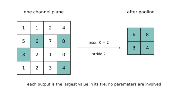
Padding is not used here, and the reason is a small piece of arithmetic rather than a convention. Pooling normally follows a ReLU, so its inputs are non-negative; padding the plane with zeros and taking a maximum over a window containing them therefore changes nothing, and the whole exercise reduces to a no-op at the border.

Two further consequences of choosing the max are worth naming. It is a non-linearity in its own right, so a convolution followed by max pooling has one whether or not a ReLU was inserted between them, whereas average pooling is linear and supplies none. And it grants a small amount of local invariance: the value 6 in Equation 6.6 can move to any of the four positions in its tile and the output is unchanged, so the layer is deliberately blind to shifts smaller than its kernel.

Interleaved with convolutions, this gives the shape of a classical convolutional network — two convolutions, a pool, two convolutions, a pool, and so on until the spatial dimensions are small, then a flatten and one or two fully connected layers to produce class scores. The next chapter is largely a history of variations on that skeleton, including the observation that a stride-2 convolution can do the same downsampling with parameters attached, which is why pooling is less ubiquitous in recent architectures than the pattern above suggests.

One practical consequence of the flatten at the end deserves flagging. The fully connected head expects a fixed number of inputs, so a network built this way accepts exactly one input resolution, and images of any other size must be resized, padded, or grouped so that each batch is internally uniform — aspect-ratio bucketing, in the larger training pipelines. It is a constraint the convolutional body does not have and the classifier head imposes, and later architectures remove it by replacing the flatten with a pooling operation over the whole spatial extent.

6.11 Equivariance

The claim that convolution and pooling respect the spatial structure of images has been used repeatedly above as an intuition. It has a precise form. Let $f$ be a convolution or a pooling layer and let $T$ shift an image some number of pixels to the side. Then

$$f(T(x)) = T(f(x)) \tag{6.7}$$

for every input $x$ — shifting the image and then applying the layer gives the same thing as applying the layer and then shifting the result. The equality holds up to boundary conditions, which is a real caveat and not an interesting one; away from the edges of a large image it is exact.

Figure 6.7: The commutative square of Equation 6.7. Both paths from the top-left to the bottom-right produce the same feature map: the operator commutes with translation. Nobody performs the shift in practice — it is a statement about what the operator is, not a step in a computation. Drawn for these notes.

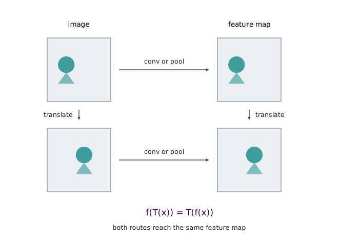
This is a property of the operator, not a preprocessing trick and not something performed during training. What makes it worth stating is that it is exactly the structural commitment Section 6.2 asked for, written down as an equation. A convolution computes each output from the same weights regardless of where in the frame it is looking, so a pattern that moves produces a response that moves with it, unchanged in value. The features an image yields depend on its content and not on where in the frame that content sits. A fully connected layer satisfies nothing of the kind: shift the input by one pixel and every dot product in the layer changes, with no relationship between the old output and the new.

Equivariance should not be confused with invariance, and the distinction organises how a network is put together. An equivariant layer’s output moves when the input moves; an invariant one’s output does not change at all. Convolution is equivariant, which is what you want in the body of a network, because a feature map that shifted with the image is still a usable description of where things are. Max pooling adds a small amount of genuine invariance, discarding shifts smaller than its window. Invariance to the whole frame arrives only at the end, from the classifier that collapses the spatial dimensions — a cat anywhere in the image should produce the same class score, but only after the layers that needed to know where it was have finished.

6.12 What this leaves

Two operators were added to the vocabulary of Section 5.11 in this chapter, and neither required anything new of the machinery. A convolution is a bank of small learned templates, applied at every position and stacked into a volume; a pooling layer reduces that volume spatially without learning anything. Both are differentiable, both fit into the computational graph beside the layers already there, and both are trained by the same loop as everything else. What distinguishes them is not their mathematics but the assumption they encode — that features are local and that location does not change meaning — which is the reason they need so few parameters to work.

What remains open is how to assemble them. The chapter has specified a layer without specifying a network: how deep, how wide, how the channel count should change as the spatial dimensions shrink, where to downsample and by how much, and whether the answers found for one problem transfer to another. Those questions were answered empirically, over roughly a decade of competition results, and the answers turned out to be more interesting than the layer. That is the next chapter.

References

• D. Lowe, “Object Recognition from Local Scale-Invariant Features,” ICCV, 1999. Paper
• Y. LeCun, L. Bottou, Y. Bengio and P. Haffner, “Gradient-Based Learning Applied to Document Recognition,” Proceedings of the IEEE, 86(11), 1998. Paper
• N. Dalal and B. Triggs, “Histograms of Oriented Gradients for Human Detection,” CVPR, 2005. Paper
• L. Fei-Fei and P. Perona, “A Bayesian Hierarchical Model for Learning Natural Scene Categories,” CVPR, 2005. Paper
• A. Krizhevsky, I. Sutskever and G. Hinton, “ImageNet Classification with Deep Convolutional Neural Networks,” NeurIPS, 2012. Paper
• J. Springenberg, A. Dosovitskiy, T. Brox and M. Riedmiller, “Striving for Simplicity: The All Convolutional Net,” ICLR, 2015. arXiv:1412.6806
• A. Vaswani et al., “Attention Is All You Need,” NeurIPS, 2017. arXiv:1706.03762
• A. Dosovitskiy et al., “An Image Is Worth 16x16 Words: Transformers for Image Recognition at Scale,” ICLR, 2021. arXiv:2010.11929
• R. Rombach, A. Blattmann, D. Lorenz, P. Esser and B. Ommer, “High-Resolution Image Synthesis with Latent Diffusion Models,” CVPR, 2022. arXiv:2112.10752