14  Generative Models I

Lecture 13

Based on Lecture 13 of CS231n, Stanford University, Spring 2025.

14.1 Two axes, not one

Almost everything in this course so far has been supervised learning. A dataset of pairs $(x, y)$, a function to be learned that maps $x$ to $y$, and a loss that measures the discrepancy on examples where the answer is known. Classification, detection, segmentation and captioning differ in what $y$ is — a category, a set of boxes, a per-pixel label, a sentence — but not in their structure. The thing you want to predict is exactly the thing your dataset records, and the work is to fit a mapping that agrees with the data and keeps agreeing on inputs it has not seen.

Unsupervised learning is described by what it lacks: there is no $y$. You have images and nothing else, and the goal is stated vaguely on purpose — find structure in the data. The vagueness is real. $k$-means finds clusters, principal component analysis finds a low-dimensional subspace that explains most of the variation, and density estimation fits a probability distribution. These are all called unsupervised, and they produce objects of entirely different kinds.

It helps to notice that they are not competing answers to one question but points along a spectrum, and that the spectrum has a direction. At one end sits density estimation: model the distribution that generated the data, in full, with nothing thrown away. At the other sits representation learning: extract from each image a short vector that retains what matters and discards the rest, where “what matters” is defined only by whatever downstream task eventually uses the vector. Clustering and PCA live near the representation end. A model that assigns a probability to every possible image lives at the density end. The previous chapter’s contrastive methods are near-pure representation learning: SimCLR never assigns a probability to an image, and could not be asked to.

Figure 14.1: The two axes the lecture separates. Supervision — whether a human produced the target — is orthogonal to what the method actually produces, which runs from a full density over the data to a short vector per example. The two families in this chapter are placed by what they compute: an autoregressive model is at the density end and offers no useful latent, while an autoencoder is at the representation end and offers no density at all. The variational autoencoder is the interesting case, because it is trying to reach both ends at once and pays for the attempt.

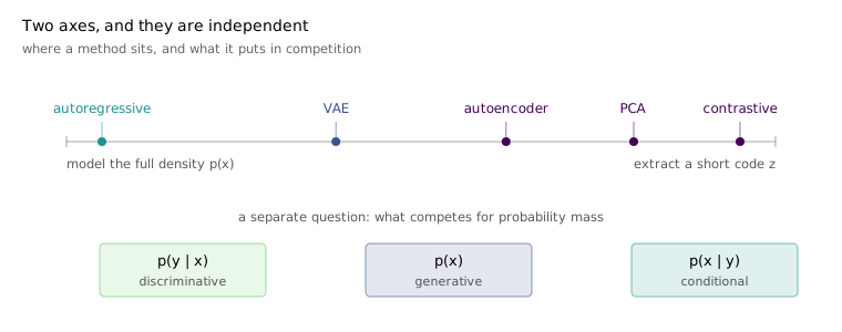
The second axis is orthogonal to the first, and it is the one this chapter is about. Cutting across supervised and unsupervised is the distinction between generative and discriminative models. This axis is inherently probabilistic: to be on it at all, a model has to commit to a probability distribution over some of its variables. Clustering and PCA sit off the axis entirely — both admit probabilistic readings, but neither requires one.

The distinction turns out to be sharper than it looks, and the reason has nothing to do with architectures.

14.2 Probability mass is a fixed budget

Write $x$ for the data — a high-dimensional thing, an image — and $y$ for a label, caption, or other comparatively small piece of side information. A discriminative model learns $p(y \mid x)$. A generative model learns $p(x)$. A conditional generative model learns $p(x \mid y)$. These are three arrangements of two symbols, and their differences look cosmetic.

They are not, and the reason is the property that makes a function a probability distribution in the first place. A density $p(x)$ assigns a non-negative number to every point in its domain subject to

$$\int p(x) \, dx = 1 . \tag{14.1}$$

The integral runs over the entire space of possible values. This single constraint is where the force of probabilistic modelling comes from, because it means there is a fixed unit of probability mass to distribute and no more. Choosing a distribution is choosing how to apportion that unit across the whole domain, and every point in the domain is therefore in competition with every other. Raising the probability of one value necessarily lowers the probability of others. There is no way to be generous to everything.

So the question to ask of any probabilistic model is: what is competing? The symbols on the page look alike; the competitions they set up do not.

In a discriminative model $p(y \mid x)$, the competition is among labels, and it is run separately for each $x$. Fix an image and the model emits a distribution over the label set — for a two-class problem, a number for cat and a number for dog that sum to one. Change the image and you get a different distribution over the same label set. Crucially, images do not compete with each other for anything. Each image induces its own budget, spends it among the labels, and is done. Nothing in the objective ever asks whether one image is more plausible than another, and nothing in the model’s output could express such a judgement.

Figure 14.2: The two competitions. On the left, a discriminative model gives each image its own budget to spend across the label set: the columns sum to one and nothing connects them, which is why the monkey must still be assigned to cat or dog. On the right, a generative model spends a single budget across the whole space of images, so the columns are no longer independent and the monkey can simply be assigned almost nothing. The difference is in which direction the bars are constrained to sum to one, and it is not a property of the architecture.

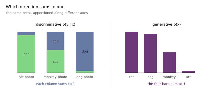
That has an immediate and slightly uncomfortable consequence: a discriminative model cannot reject its input. Fix the label vocabulary at cat and dog, feed the trained model a photograph of a monkey, and it is structurally obliged to answer with a distribution over cat and dog. It has nowhere to put the mass. It cannot say that the question does not apply, because Equation 14.1 is enforced along the label axis and the label axis contains no such option. This is not a training failure to be fixed with more data. It is the shape of the model.

A generative model $p(x)$ moves the competition. Now every image that could exist is competing with every other for one unit of mass, and the model gains exactly the capacity the discriminative one lacked: it can assign an input a probability near zero, which is a statement that the input is not the kind of thing this model is about. A density fitted to photographs of zoo animals should give a piece of abstract art essentially nothing, and that is a meaningful output rather than a refusal to answer.

The capacity is bought at a steep price, and it is worth being explicit about how steep. Apportioning mass across all possible images forces the model to answer questions it would rather avoid. Should an image of a three-legged dog receive more mass than an image of a three-armed monkey? Probably yes — a dog can lose a leg, and there is no comparable route to a third arm — but arriving at that answer requires something like a model of how the world produces the images it produces. The problem stated in one line, $\int p(x)\,dx = 1$, quietly contains most of visual understanding.

Conditional generative models are the arrangement that matters in practice, and they compound the difficulty in an interesting direction. For every value of $y$, the model induces a separate competition among all images. Conditioned on cat, the cat photograph should be high, the dog and monkey photographs middling — they are at least animals — and the abstract art near zero; conditioned on dog, a different apportionment of the same total. When $y$ is a category label this is a modest generalisation. When $y$ is a paragraph of text, or an image plus a piece of text, the model is being asked to place a distribution over all images for every point in an enormous and richly structured conditioning space, which is a problem with no clean specification at all. All that changed from the discriminative case was the position of two symbols.

14.3 Bayes’ rule connects all three

The three arrangements are not independent objects. They are related by

$$p(x \mid y) = \frac{p(y \mid x)\, p(x)}{p(y)}, \tag{14.2}$$

which says that a discriminative model, an unconditional generative model, and a prior over labels together determine a conditional generative model. The identity rearranges, so any two of the pieces give you the third. In principle you never need to train a conditional generative model: train a classifier, train a density over images, count label frequencies, and multiply.

In practice nobody does this, and conditional generative models are trained directly from scratch. The reason is that Equation 14.2 is exact about the relationship and silent about the difficulty — it requires an unconditional $p(x)$ that is accurate enough to divide by, which is the hardest of the three objects to obtain. The relationship is still worth carrying, partly because it is the cleanest statement of how the families connect, and partly because it does get used: classifier-free guidance in diffusion models trains conditional and unconditional models jointly and combines their predictions at sampling time, which is Equation 14.2 doing real work rather than serving as a remark.

14.4 What a density is actually for

Discriminative models need no justification here; the whole course to this point has been their applications. Train one and you can assign labels, and the features it learns along the way transfer to tasks it was never shown, which is the transfer learning of Section 7.12.

Unconditional generative models are harder to defend, and the honest assessment is that on their own they have not turned out to be very useful. They give you outlier detection, which is a real if narrow application of the rejection capacity from the previous section. They give you a form of representation learning that needs no labels — the hope being that fitting $p(x)$ forces the model to learn something about images along the way — and the record there is poor: the contrastive methods of the previous chapter beat unconditional density estimation at producing transferable features, consistently and by a wide margin. And they give you samples. But a sample from $p(x)$ is an image you had no say in. The model hands you something plausible and you take what you are given, which makes unconditional sampling a mathematically interesting capability with very little practical purchase.

Conditional generative models are where nearly all of the value is, and it comes almost entirely from sampling. If $y$ is a piece of text then sampling from $p(x \mid y)$ is text-to-image generation, and the conditioning is precisely the control that unconditional sampling lacks. You can also in principle classify with rejection — evaluate $p(x \mid y)$ across all $y$ and decline to answer if every one is low — though this is rare in practice. The thing that is not rare, and that motivates the two chapters on generative models, is controllable synthesis.

There is a caveat worth attaching to the dismissal of unconditional models, because the field has partly overturned it since. Large language models are trained as unconditional density estimators over token sequences; the conditioning that makes them useful is supplied at sampling time by fixing a prefix, not by a separate conditioning pathway during training. The clean split between conditional and unconditional is a statement about how the distribution is factored, not about whether the model can be steered, and the sharpest counterexample to “unconditional models are useless” is the most commercially significant class of generative model in existence.

14.5 A taxonomy by what you can compute

The useful way to organise generative models is not by architecture. It is by which operations the model actually supports, because the operations turn out not to come as a package.

There are two you might want. You might want to evaluate the density: hand the model an $x$ and get a number. You might want to sample: ask the model for a fresh $x$ drawn from what it has learned. It is tempting to assume that anything which can do one can do the other — a distribution is a distribution — but the two are computationally quite different requests, and every generative model in use makes a trade between them.

Models that can return $p(x)$ for an input are explicit density models. Models that cannot, but can produce samples, are implicit density models: the density has been learned in the sense that the samples are distributed according to it, but there is no way to read the value out. That sounds like a pure loss, and it is often not, because for the applications that matter most you may genuinely not care what number the density assigns to any particular image. If all you want is a stream of good, varied samples, the ability to evaluate is a luxury. Meanwhile the explicit models are the ones for which sampling tends to be awkward, which is the reverse of what one would guess.

Each branch splits again, and this is the taxonomy Goodfellow’s tutorial laid out, adapted. Among explicit models, some return the tractable density — the actual $p(x)$ the model defines, exactly, with no approximation. Autoregressive models are the example and they are the first half of this chapter. Others return an approximate density: a number that is not $p(x)$ but a computable bound on it. Variational autoencoders are that case, and they are the second half. Among implicit models, some sample directly — one forward pass of a network produces a sample, which is what a generative adversarial network does. Others sample indirectly, through an iterative procedure with no single feed-forward route to a sample. Diffusion models are the case, and they occupy the next chapter.

Figure 14.3: The four leaves, arranged by what the model will do for you. The first split is whether a density value is obtainable at all; the second, on each side, is whether it is the true one and whether sampling is a single pass. Note that the two dimensions are not aligned: the leaf that gives you an exact density is the one that samples most slowly, and the leaf that samples in one pass gives you no density at all.

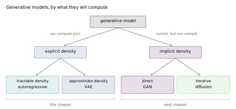
The distinction between the approximate-density leaf and the indirect-implicit leaf is worth stating carefully, because they can both be described as “you get something less than the real density”. In the approximate case there is a number, and it is a bound on the true $p(x)$; you can compute it, compare it across inputs, and use it as a training objective. In the indirect implicit case there is no density value anywhere in the model to be found, and the only thing on offer is a sampling procedure. And the iterative procedure cannot be wrapped up and treated as a direct sampler, because the iteration converges to a true sample only in the limit. Diffusion sampling with finitely many steps gives an approximate sample, and the same was true of the Markov-chain methods that preceded it.

One notational habit to absorb before going further, because the lecture flags it and every paper in this area relies on it. Everything from here is written $p(x)$, unconditionally. The conditioning on $y$ is dropped for readability, not because it is absent: every density, objective and bound below has a $\mid y$ that can be reinstated wherever it is wanted, and in the models people actually deploy it is there. Read $p(x)$ as $p(x \mid y)$ with the label suppressed.

14.6 Maximum likelihood, and the direction of the divergence

Suppose the model is a neural network that takes an image $x$ and weights $W$ and returns a density, $p(x) = f(x, W)$. Given a dataset $x^{(1)}, \ldots, x^{(N)}$, how should $W$ be chosen? The answer that organises essentially all of explicit generative modelling is to pick the weights under which the data you actually observed is most likely:

$$W^* = \arg\max_W \prod_{i=1}^{N} p\big(x^{(i)}\big) = \arg\max_W \sum_{i=1}^{N} \log f\big(x^{(i)}, W\big). \tag{14.3}$$

The product over $i$ assumes the samples are independent and identically distributed, so the joint density of the dataset factors. The step to the sum is the log trick, and it earns its place twice over: $\log$ is monotonic, so maximising the log of a quantity maximises the quantity, and it turns the product into a sum, which gradient descent handles and which does not underflow. In practice you will rarely see a density value in an implementation at all — models emit log-probabilities, losses are computed in log space, and this is for numerical survival rather than elegance. Superscripts index samples throughout; subscripts, from the next section, index parts of a single sample.

The word “likelihood” rather than “probability” marks what is being varied. Probability fixes the distribution and varies $x$: how much mass does this fixed density put on this point? Likelihood fixes the observed $x$ and varies the distribution: among all the densities the network can express, which makes these particular samples least surprising? The equation is the same; the argument to the optimisation is not.

Underneath the whole exercise is an assumption that deserves saying out loud. There is a true distribution $p_{\text{data}}$ from which the world drew the images you have. You cannot see it, and never will — you have a finite sample from it and nothing more. Maximum likelihood is one procedure for guessing at it from that sample, and it is worth knowing exactly what kind of guess it makes.

Take the average of Equation 14.3 over the dataset and let $N$ grow, so the empirical average converges to an expectation under $p_{\text{data}}$:

$$\frac{1}{N}\sum_{i=1}^{N} \log p_\theta\big(x^{(i)}\big) \;\longrightarrow\; \mathbb{E}_{x \sim p_{\text{data}}}\big[\log p_\theta(x)\big] = -H(p_{\text{data}}) - D_{\mathrm{KL}}\big(p_{\text{data}} \,\|\, p_\theta\big). \tag{14.4}$$

The entropy $H(p_{\text{data}})$ is a property of the world and does not depend on $\theta$, so maximising likelihood is exactly minimising the Kullback–Leibler divergence from the data distribution to the model. That is a satisfying justification, and it also carries a warning, because KL divergence is asymmetric and Equation 14.4 fixes which direction you get. The expectation is taken under $p_{\text{data}}$, which means the model is punished savagely wherever the data has mass and the model does not — $\log p_\theta(x) \to -\infty$ — and not punished at all wherever the model has mass and the data does not. The objective is mode-covering: it insists the model cover everything the data does, and it is indifferent to mass spent on things the data never produces.

Figure 14.4: The best single Gaussian fit to a bimodal target, under each direction of the KL divergence. Both fits are computed in the generator, the forward-KL one by moment matching (which is what minimising $D_{\mathrm{KL}}(p \| q)$ over Gaussians reduces to) and the reverse-KL one by grid search over the objective, restricted to the right-hand mode since a symmetric target gives that direction two equivalent optima. Maximum likelihood gives the left panel: rather than commit to either mode, it spreads across both and puts substantial mass in the valley between them, where the data has almost none. When the model is a decoder over images, mass in the valley is what an average of two plausible images looks like, which is to say a blurry one.

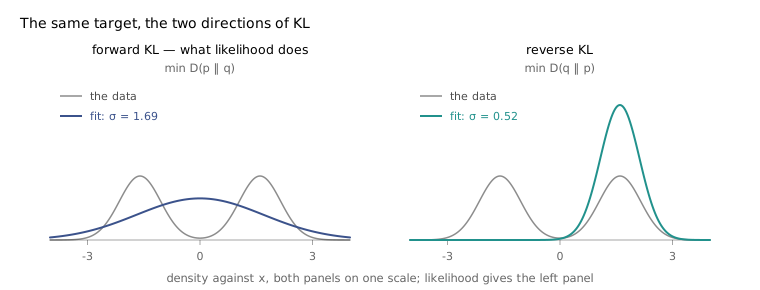
This is not a technicality to file away. Every likelihood-trained generative model inherits the mode-covering bias, and it is the standard explanation for why models in this family produce samples that are blurry and slightly averaged rather than sharp and occasionally wrong. Adversarial models, which optimise something closer to the other direction, have the complementary failure: sharp samples, and whole modes of the data silently missing.

14.7 The chain rule needs no assumptions

Maximum likelihood tells you what to maximise but not how to write down $f(x, W)$ so that its output is a normalised density. That is the real difficulty, and it is where the model families diverge.

The autoregressive answer is to assume the data has a canonical decomposition into an ordered sequence of parts, $x = (x_1, x_2, \ldots, x_T)$, and then apply the chain rule of probability:

$$p(x) = p(x_1, x_2, \ldots, x_T) = \prod_{t=1}^{T} p\big(x_t \mid x_1, \ldots, x_{t-1}\big). \tag{14.5}$$

The remarkable thing about Equation 14.5 is that it assumes nothing. It is not a modelling approximation, not a conditional independence claim, not a factorisation that discards interactions. It is an identity, true of every joint distribution over every set of random variables. The only commitment is the choice of ordering, and the identity holds for any ordering you pick.

What the factorisation buys is that each factor is small. To see why that matters, count. For a vocabulary of $V$ tokens, the joint distribution over a sequence of $T$ of them is a table with $V^T$ entries — a hundred thousand words and a twenty-token sentence puts the table beyond any conceivable representation. The factored form never asks for that table. It asks for one distribution over $V$ options at a time, conditioned on a prefix, and the network’s job is to map prefixes to $V$-way distributions. Exponential becomes linear in $T$, and the price is that the conditioning is now the network’s problem rather than the table’s.

And a network that maps a prefix to a distribution over the next element is something this course has already built twice. An RNN carries a hidden state forward that summarises the sequence so far and emits a distribution over the next element at each step, which is exactly Equation 14.5 with $h_t$ standing in for $x_1, \ldots, x_{t-1}$ — the language model of Section 8.6 was an autoregressive generative model, described in different vocabulary. A Transformer with a causal attention mask does the same thing without the recurrence: masking the attention matrix so position $t$ attends only to positions $\le t$ is precisely the constraint Equation 14.5 requires, as Section 9.11 set out. This is what a large language model is. There is no additional generative machinery — the next-token objective is maximum likelihood under a chain-rule factorisation, and the cross-entropy loss the model is trained with is $-\log p(x)$ summed over positions.

That correspondence makes the exactness concrete. Push a sequence through a trained Transformer once. At every position it has emitted a distribution over the vocabulary conditioned on the prefix; read off the probability it assigned to the token that actually occurred, and multiply across positions. The result is $p(x)$ for that sequence — not a bound, not an estimate, the value the model defines. One forward pass, and you have the exact density. This is what puts autoregressive models in the tractable-density leaf of Figure 14.3.

Sampling is the other direction and it is not symmetric. To draw a sample you have nothing to condition on, so you must generate $x_1$ from the model, feed it back, generate $x_2$ from the extended prefix, feed that back, and continue. Each step needs the previous step’s output, so the $T$ network evaluations are irreducibly sequential. Training parallelises perfectly — every position’s target is known in advance, so one pass computes all $T$ losses at once — and sampling parallelises not at all. That asymmetry is the defining property of the family, and for text, where $T$ is a few thousand, it is an inconvenience.

14.8 Images do not come as sequences

Text fits Equation 14.5 almost suspiciously well. It is already one-dimensional, so the ordering is given rather than chosen, and it is already discrete, so each factor is a distribution over a finite vocabulary — which is to say a softmax, trained with cross-entropy, exactly the machinery this course has used since the second lecture.

Images have neither property. They are two-dimensional, so any ordering is imposed rather than found, and they are ordinarily thought of as continuous. The second objection is the easier one to dissolve, and the dissolution is worth appreciating for how blunt it is: images as actually stored are not continuous. A PNG or JPEG holds eight bits per channel, so a pixel is three integers in $[0, 255]$ and nothing else. The continuity was an idealisation the file format never had.

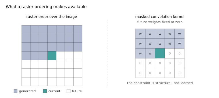
So an image can be flattened into a sequence in raster order — left to right along each row, top to bottom down the rows, and within each pixel the three channels in a fixed order — giving a one-dimensional sequence of discrete symbols with a vocabulary of 256. Every tool from the previous section now applies unchanged. This is PixelRNN and PixelCNN, which predict each subpixel as a 256-way classification and differ in how the prefix is summarised: the recurrent versions carry LSTM state across the image, and PixelCNN uses masked convolutions, where the mask zeroes the kernel weights that would otherwise read pixels later in the raster order.

Figure 14.5: The causal structure a raster ordering imposes. Everything above the current pixel’s row is available, along with everything to its left in the same row; everything to its right and below is not, regardless of how close it is. The masked convolution on the right is how this is enforced in a convolutional model: the kernel’s weights over the future half of its footprint are held at zero, so the constraint is structural rather than something the network has to learn. The pixel immediately below the current one is a nearer neighbour than the one at the far end of the previous row, and the ordering makes it unavailable anyway.

The approach works, in the sense that it produces genuine likelihood numbers and they are good. Density on images is conventionally reported in bits per dimension — the negative log-likelihood per subpixel in base two, which is directly the number of bits an optimal compressor built from the model would spend. It is a scale with meaningful landmarks at both ends. A model that has learned nothing and treats every subpixel as uniform over 256 values costs exactly 8 bits per dimension. A full multivariate Gaussian fitted to CIFAR-10 gets to 4.70. PixelCNN reaches 3.14, and the strongest of the recurrent variants 3.00, against a previous state of the art of 3.47.

Figure 14.6: CIFAR-10 test-set density in bits per dimension, from Table 5 of the PixelRNN paper, with the uniform baseline at exactly 8 bits marking what no modelling at all costs. Lower is better and the axis does not start at zero, because the interesting comparison is among the models rather than against the baseline. The ordering of the three PixelRNN variants tracks the size of the context each one can see, which is the paper’s own explanation for the gap.

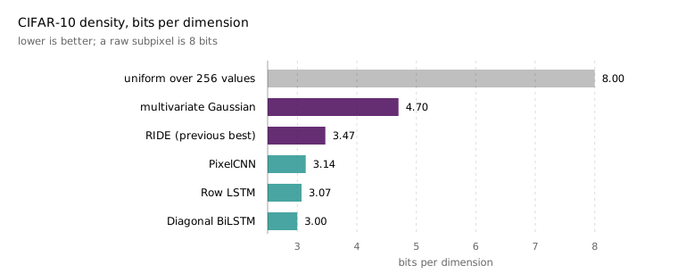
The internal ordering of those results is the more informative part. The three variants rank exactly as their receptive fields do: the bidirectional diagonal model, which can see the entire available prefix, beats the row-wise model, which sees a partially occluded prefix, which beats PixelCNN, which sees the least. Depth pushes in the same direction and saturates slowly: on the validation split the row-wise model goes from 3.30 bits per dimension with one layer to 3.06 with twelve. Both observations say the same thing — the bottleneck is how much of the prefix the model can actually condition on — and that is a reassuring thing to find, because it means the numbers are measuring the model’s grasp of long-range structure rather than an artefact of the parameterisation.

Then there is the problem that killed the approach. Sampling requires one network evaluation per element, sequentially, and an image has a great many elements. A $32 \times 32$ colour image is a sequence of 3,072 subpixels, so a single sample costs 3,072 forward passes. That is tolerable, and it is why the published results are at $32 \times 32$ and $64 \times 64$ — where the paper reports 3.86 and 3.63 bits per dimension — rather than anywhere near a useful resolution. Go to $1024 \times 1024$, which is a good but hardly extravagant resolution, and the sequence is 3,145,728 subpixels long. Every one of those forward passes waits for the one before it.

Figure 14.7: Sequential decoder evaluations required for one sample, against image side length, for a three-channel image at one network pass per subpixel. Both axes are logarithmic. The two resolutions the PixelRNN paper reports results at are marked, along with the resolution a text-to-image model is expected to produce today; the cost is quadratic in side length, so the gap between them is four orders of magnitude and no amount of hardware closes it, because the passes cannot be run in parallel.

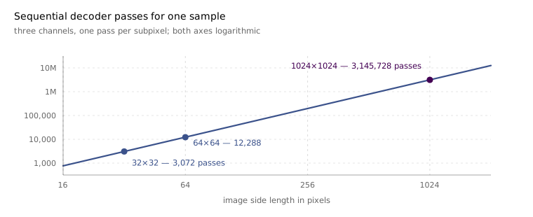
Sequences of a few million elements are not beyond current models. But paying a few million sequential network evaluations for one image is not a practical generative model, and it is the reason autoregressive modelling of raw pixels was largely abandoned. The family came back — most of the strong image and video generators of the last few years are autoregressive somewhere inside — but not over pixels. The move that rescued it was to stop treating the raster as the sequence and instead learn a compression from images to a much shorter sequence of discrete tokens, then be autoregressive over those. The next chapter takes that up.

There is a second, quieter objection worth registering, because it is conceptual rather than computational. The raster ordering is arbitrary. Nothing about images makes left-to-right, top-to-bottom the right decomposition, and Equation 14.5 is exact for any ordering, which means the model is free to be wrong about which pixels are near each other and the mathematics will not object. The pixel directly below the current one is a close neighbour in the image and a distant one in the sequence, and a model conditioning on a raster prefix has to rediscover through its weights a spatial structure the ordering destroyed. That the convolutional variants do worse than the recurrent ones despite having the better spatial prior is a hint at how much is being asked here.

14.9 Reconstruction without a distribution

The second family in this chapter gives up something the first had and gets something the first lacked. Autoregressive models compute the exact density and hand you no representation of an image beyond the image itself; there is no vector in a PixelCNN that summarises what it is looking at. Variational autoencoders trade exactness for a latent space — an explicit, low-dimensional code per image, arriving as a by-product of the training — and the trade is worth making often enough that the family has outlasted its likelihood numbers.

Getting there needs the non-probabilistic version first, since the course has not built one. Take an encoder network — any architecture, a convolutional network is typical — mapping an image $x$ to a vector $z$. Take a decoder mapping $z$ back to an image $\hat{x}$. Train the pair so that $\hat{x}$ matches $x$ under an $L^2$ loss.

Stated that baldly it is a strange thing to do. The objective is to approximate the identity function, which is already known, using an expensive network trained on a large dataset. The point is entirely in the constraint: $z$ is made much smaller than $x$. A $1024 \times 1024$ colour image is about three million numbers and $z$ might be 128 of them, so the network cannot pass the image through and must instead find a description short enough to fit and informative enough to reconstruct from. With an unconstrained $z$ the problem is trivial and the model learns nothing; the bottleneck is what converts a pointless objective into a useful pressure. Principal component analysis is the linear special case of exactly this, which is a good way to see what the bottleneck is doing — finding the subspace that loses the least — and how much a nonlinear encoder adds.

Figure 14.8: What an autoencoder gives you and what it does not. Reconstruction constrains the encoder and decoder along the paths drawn solid, and the codes that training produces occupy some region of latent space whose shape nothing in the objective controls. Sampling requires knowing that region, and the loss never says a word about it: a vector drawn at random from the latent space is overwhelmingly likely to land where no training image ever mapped, and the decoder has no obligation to do anything sensible there.

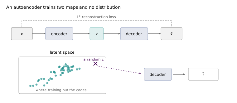
Trained, an autoencoder can be used in the manner of the previous chapter: discard the decoder, keep the encoder, attach a head, fine-tune on whatever labels you have. It is a self-supervised method, and the reconstruction objective is a pretext task with no shortcut available.

To generate, you would want the opposite operation — discard the encoder, sample a $z$ from somewhere, and decode it. This would be an implicit generative model of the kind Section 14.5 described: samples with no density value anywhere. And it does not work, for a reason that is easy to state and easy to underestimate. There is no distribution over $z$. Nothing in the reconstruction loss says anything about where in latent space the codes live, how they are spread, or what lies between them. Training maps each image somewhere and is indifferent to the geometry of the result, so a vector drawn from any distribution you care to name will almost certainly not resemble any code the encoder ever produced, and the decoder — never trained on such input — will return something incoherent.

Notice that this is not progress disguised as a problem. The original difficulty was that we did not know how to sample images. The autoencoder converts it into the difficulty of sampling latent codes, which is a smaller space but not a better-understood one. The can has been kicked down the road.

The variational autoencoder’s idea is to stop hoping the latent space will turn out to have a convenient shape and instead make it have one. Add to the objective a term that pushes the codes towards a distribution chosen in advance — a unit Gaussian, in practice essentially always — and then sampling is trivial by construction: draw $z \sim \mathcal{N}(0, I)$, decode, done. The rest of this chapter is the work of making that idea into something trainable, and the work is more interesting than the idea.

14.10 One latent variable, two intractable integrals

Set up the generative story properly, as a claim about how the data came to exist. For each observed image $x^{(i)}$ there was a latent vector $z^{(i)}$ that came first, and the image was generated from it. The latent vector contains everything needed to produce the image — the identity of the objects, their number, their pose, the lighting — and it is never observed. There is no dataset of $z$’s, and there never will be.

Two distributions define the model. The prior $p(z)$ is chosen, not learned, and is taken to be $\mathcal{N}(0, I)$. The decoder $p_\theta(x \mid z)$ is a neural network with weights $\theta$. Together they specify a distribution over images, and if the $z^{(i)}$ were observed, fitting them would be ordinary maximum likelihood on pairs — precisely the conditional generative modelling of Section 14.2.

They are not observed, so the thing to maximise is the marginal, with $z$ integrated out:

$$p_\theta(x) = \int p_\theta(x \mid z)\, p(z) \, dz . \tag{14.6}$$

Every symbol in Equation 14.6 is available. The decoder is a network we can evaluate; the prior is a Gaussian we can write down. And the expression is nonetheless useless, because the integral is over the whole latent space and the integrand runs through a neural network. There is no analytic solution and no reason to expect one. Nor does numerical integration rescue it: $z$ has enough dimensions that quadrature is hopeless, and while the integral is an expectation under the prior that could in principle be estimated by sampling, the estimate has ruinous variance — the prior places almost none of its mass in the region where $p_\theta(x \mid z)$ is large for a given $x$, so nearly every sample contributes nothing. Putting a high-variance Monte Carlo estimate inside the inner loop of training is not a plan.

Try Bayes’ rule instead, which is the other move available. Rearranging Equation 14.2 for this model,

$$p_\theta(x) = \frac{p_\theta(x \mid z) \, p(z)}{p_\theta(z \mid x)}, \tag{14.7}$$

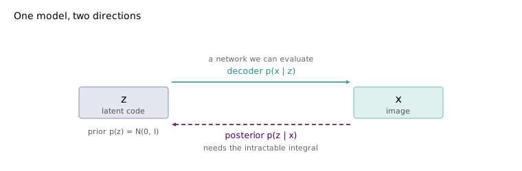
which is an improvement in one respect — no integral — and a dead end in another. The numerator is fine: decoder and prior. The denominator is the posterior $p_\theta(z \mid x)$, the distribution over latent codes that could have produced a given image, and computing it requires exactly the integral from Equation 14.6 as its normalising constant. The two intractabilities are one intractability seen from two sides.

Figure 14.9: The two directions, and which of them the model actually contains. The generative direction, drawn solid, is what the model defines: a prior over codes and a decoder that turns a code into a distribution over images. The inference direction, drawn dashed, is what Equation 14.7 needs and what no part of the model provides — recovering the code that produced an image requires inverting the decoder, and a neural network is not invertible. The whole of the next section is a response to the dashed arrow.

14.11 A second network for the posterior

The move that makes the variational autoencoder work is to give up on computing $p_\theta(z \mid x)$ and approximate it with another neural network. Introduce $q_\phi(z \mid x)$ — separate weights $\phi$, trained jointly with $\theta$ — whose job is to output, for an image, a distribution over the latent codes that plausibly produced it. It approximates the posterior, and nothing forces the approximation to be good; the derivation in the next section will tell us exactly what the failure costs.

This gives the architecture its two halves and its name. The decoder $p_\theta(x \mid z)$ takes a code and returns a distribution over images. The encoder $q_\phi(z \mid x)$, also called the recognition model, takes an image and returns a distribution over codes. Compared with Section 14.9, both halves have been made probabilistic: each now emits a distribution rather than a point.

Which raises a mechanical question. A network outputs numbers, and a distribution is a function — how does the first produce the second? By fixing the family in advance and having the network output its parameters. Both halves here are Gaussian with diagonal covariance, so the encoder emits two vectors of the same length as $z$: a mean $\mu_{z \mid x}$ and a diagonal standard deviation $\sigma_{z \mid x}$, together specifying $\mathcal{N}(\mu_{z \mid x}, \operatorname{diag}(\sigma_{z\mid x}^2))$.

The diagonal restriction is not a matter of taste. A full covariance over a $d$-dimensional latent space needs $d(d+1)/2$ outputs and must be positive semi-definite, which is an awkward thing to guarantee from a network’s raw output. Diagonal needs $d$ outputs, is positive by construction if the network emits a log standard deviation, and — the reason that actually matters — makes the divergence against the prior available in closed form. The cost is that the encoder cannot express any correlation between latent dimensions. That cost buys something back in Section 14.14, where the independence turns out to be the mechanism behind the family’s most attractive property.

The decoder is handled slightly differently, and the asymmetry is worth understanding because it explains why implementations look nothing like the equations. The decoder is also nominally a diagonal Gaussian, this time over pixels, with the network emitting the mean $\mu_{x \mid z}$ and the variance held fixed at some constant $\sigma^2$ rather than predicted. Fixing it is the right call. A predicted per-pixel variance with no correlation structure would say that each pixel independently wobbles by its own amount, and sampling from that distribution means taking the mean image and adding independent per-pixel noise — which is not a sensible model of how images vary, and produces speckle rather than plausible alternatives. So in practice the decoder’s distribution is a fiction maintained for the derivation: at sampling time the mean is simply output, and nothing is ever drawn from it.

The fiction pays for itself immediately. With variance fixed, the log-likelihood of a Gaussian is

$$\log p_\theta(x \mid z) = -\frac{\lVert x - \mu_{x \mid z} \rVert^2}{2\sigma^2} + \text{const}, \tag{14.8}$$

so maximising it is minimising squared error between the decoder’s output and the input, with $\sigma^2$ absorbed into a weight on the term. The probabilistic reconstruction objective is the $L^2$ loss of an ordinary autoencoder. The whole apparatus of distributions produces, at the point of implementation, the loss you would have written anyway.

14.12 The evidence lower bound

Now the derivation. It is one page of manipulation and it earns close reading, because the term that gets discarded at the end is what the entire method’s approximation consists of.

Start from the objective — maximum likelihood, as always — and rewrite the marginal using Equation 14.7:

$$\log p_\theta(x) = \log \frac{p_\theta(x \mid z)\, p(z)}{p_\theta(z \mid x)} . \tag{14.9}$$

This holds for every $z$, since the right-hand side is secretly independent of $z$. Now multiply the fraction above and below by $q_\phi(z \mid x)$, which changes nothing, and split the logarithm into three terms in a particular arrangement:

$$\log p_\theta(x) = \underbrace{\log p_\theta(x \mid z)}_{\text{reconstruction}} \;-\; \underbrace{\log \frac{q_\phi(z \mid x)}{p(z)}}_{\text{prior}} \;+\; \underbrace{\log \frac{q_\phi(z \mid x)}{p_\theta(z \mid x)}}_{\text{gap}} . \tag{14.10}$$

Still an exact equality, and still true for every $z$. Next comes the step that makes the derivation work, and it is entirely legitimate while looking like sleight of hand. The left-hand side does not depend on $z$. Anything that does not depend on $z$ is unchanged by taking an expectation over $z$, under any distribution whatsoever — so take the expectation under $q_\phi(z \mid x)$, which is the distribution the encoder happens to produce. Expectation is linear, so it passes through to each of the three terms, and the second and third then match the definition of the Kullback–Leibler divergence exactly:

$$\log p_\theta(x) = \mathbb{E}_{z \sim q_\phi(z \mid x)}\big[\log p_\theta(x \mid z)\big] - D_{\mathrm{KL}}\big(q_\phi(z \mid x) \,\|\, p(z)\big) + D_{\mathrm{KL}}\big(q_\phi(z \mid x) \,\|\, p_\theta(z \mid x)\big). \tag{14.11}$$

Read the terms. The first is reconstruction, spelled out as a procedure: encode $x$ to get a distribution over codes, draw a $z$ from it, decode, and ask how much probability the decoder assigns to the original $x$. By Equation 14.8 this is squared reconstruction error. The second compares the distribution the encoder produces for this image against the prior we chose, and it is the term that shapes the latent space — the mechanism Section 14.9 said was missing, now written down. The third measures how far the encoder is from the true posterior, and it is the term we cannot compute, because $p_\theta(z \mid x)$ is exactly the object whose intractability started all of this.

So discard it. A KL divergence is non-negative whether or not you can evaluate it, so dropping the third term can only decrease the right-hand side:

$$\log p_\theta(x) \;\ge\; \mathbb{E}_{z \sim q_\phi(z \mid x)}\big[\log p_\theta(x \mid z)\big] - D_{\mathrm{KL}}\big(q_\phi(z \mid x) \,\|\, p(z)\big) \;=\; \mathcal{L}(\theta, \phi; x). \tag{14.12}$$

$\mathcal{L}$ is the evidence lower bound, or ELBO, and it is what a variational autoencoder maximises. Both terms are computable: the first from a forward pass through encoder and decoder, the second in closed form because both distributions are diagonal Gaussians. Maximising a lower bound does not maximise what it bounds, and this is the approximation the family is named for — this is why Figure 14.3 puts variational autoencoders under approximate rather than tractable density.

Figure 14.10: The decomposition of Equation 14.11, evaluated in closed form. The generator uses a one-dimensional model in which the marginal, the true posterior, and all three terms have analytic expressions, so the identity can be checked rather than asserted: the bound plus the gap reproduces $\log p(x)$ exactly. The right-hand column shows what happens as the encoder’s output is moved away from the true posterior — the bound falls and the gap opens by precisely the amount the bound lost, since their sum is a constant the encoder cannot affect.

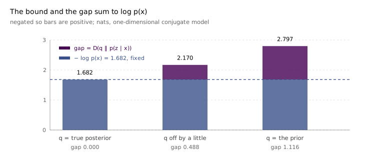
The discarded term is worth one more sentence, because it is the most informative thing in the derivation. The gap between the bound and the true log-likelihood is $D_{\mathrm{KL}}(q_\phi(z \mid x) \| p_\theta(z \mid x))$ — not bounded by it, equal to it. So the bound is tight exactly when the encoder equals the true posterior, and it is loose in proportion to how wrong the encoder is. That reframes what the encoder is for. It looks like a piece of machinery for making training possible; it is also the thing that determines how much of the actual likelihood the objective is able to see, and every restriction placed on it — the diagonal covariance above, most obviously — puts a floor under the gap that no amount of training will lift.

14.13 Getting a gradient through a sample

One obstacle remains between Equation 14.12 and a training loop. The reconstruction term is an expectation over $z \sim q_\phi(z \mid x)$, estimated in practice by drawing a single sample. That sample depends on $\phi$, since $\phi$ produced the distribution it came from — but sampling is not a differentiable operation, and backpropagation cannot pass a gradient through it. The encoder would receive no gradient from the reconstruction term at all, which is most of the objective.

The fix is to move the randomness out of the path. Rather than drawing $z$ from $\mathcal{N}(\mu_{z \mid x}, \operatorname{diag}(\sigma_{z \mid x}^2))$, draw $\epsilon$ from a fixed standard normal and construct

$$z = \mu_{z \mid x} + \sigma_{z \mid x} \odot \epsilon, \qquad \epsilon \sim \mathcal{N}(0, I). \tag{14.13}$$

The distribution of $z$ is identical. What changes is the computation graph: $\epsilon$ is now an input, drawn from a distribution with no parameters, and $z$ is a differentiable function of $\mu$, $\sigma$ and $\epsilon$. The gradient flows to $\mu$ and $\sigma$ and onward into the encoder, while the stochasticity sits on a leaf where it cannot block anything.

Figure 14.11: Why Equation 14.13 is necessary. On the left the sampling operation sits between the encoder’s outputs and the code, and the backward path stops there. On the right the same distribution is realised as a deterministic function of the encoder’s outputs and an independent noise input, and the backward path reaches the encoder through the multiplication and the addition. The two forward passes are distributionally identical; only one of them can be trained.

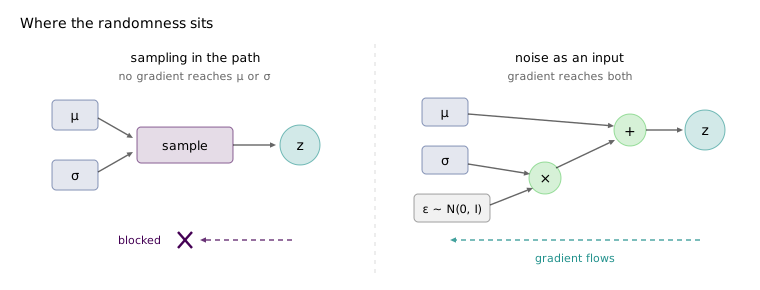
This is the reparameterisation trick, and it is the technical contribution that made the whole framework practical. It was introduced by Kingma and Welling and, independently and simultaneously, by Rezende, Mohamed and Wierstra under the name stochastic backpropagation. The ELBO itself had been known in variational inference for years; what these papers supplied was the means to optimise it with the same gradient machinery as everything else, at which point the encoder and decoder could be arbitrary neural networks.

The training step is now unremarkable. Push $x$ through the encoder to get $\mu_{z\mid x}$ and $\sigma_{z\mid x}$; evaluate the prior KL in closed form from those two vectors; draw $\epsilon$ and form $z$ by Equation 14.13; push $z$ through the decoder; compute squared error against $x$; add the two terms and take a gradient step in $\theta$ and $\phi$ together. Every part of that is a standard operation, which is the point of the preceding four sections.

14.14 Two terms that want opposite things

The most interesting property of Equation 14.12 is that its two terms disagree, and the disagreement is not a defect to be tuned away — it is the mechanism.

Consider what each term would do if it were alone. The reconstruction term wants $\sigma_{z \mid x} \to 0$ and a distinct $\mu_{z\mid x}$ for every image. With zero variance the code is deterministic, the sampling step does nothing, and the model is free to assign each training image its own private point in latent space and reconstruct it perfectly. Reconstruction alone turns a variational autoencoder back into the ordinary autoencoder of Section 14.9, with all of that section’s problems.

The prior term wants the opposite: $\mu_{z\mid x} \to 0$ and $\sigma_{z\mid x} \to 1$ for every image, because that is when $q_\phi(z \mid x)$ matches $\mathcal{N}(0, I)$ and the divergence vanishes. Prior alone produces an encoder that ignores its input entirely and a latent space that is perfectly shaped and carries no information.

Neither extreme is what you want, and the useful model is wherever they balance. It is worth doing the balance exactly, because in one dimension it can be done in closed form and the answer is more informative than the qualitative story. Take $p(z) = \mathcal{N}(0, 1)$ and a decoder $p(x \mid z) = \mathcal{N}(z, \sigma_x^2)$ — a decoder that passes the code through and adds noise of scale $\sigma_x$, which stands in for how much of the image the code fails to determine. Maximising Equation 14.12 over $\mu_q$ and $\sigma_q$ then gives

$$\mu_q = \frac{x}{1 + \sigma_x^2}, \qquad \sigma_q^2 = \frac{\sigma_x^2}{1 + \sigma_x^2}, \tag{14.14}$$

which are exactly the mean and variance of the true posterior $p(z \mid x)$. The two terms fighting to a draw land on the right answer, the gap in Equation 14.11 closes to zero, and the bound becomes tight — the derivation and the tension are the same fact viewed twice.

Figure 14.12: The two terms of the ELBO as functions of the encoder’s predicted standard deviation, for the one-dimensional model above. Reconstruction cost falls monotonically as the code becomes more deterministic; the prior term has its minimum at $\sigma_q = 1$ and rises steeply as $\sigma_q \to 0$, because the logarithm in the Gaussian KL diverges there. Their sum has an interior minimum at the value Equation 14.14 predicts, marked, and the generator solves for it numerically as a check on the closed form.

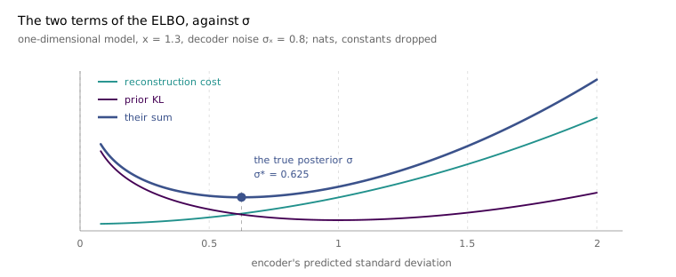
Equation 14.14 also explains the family’s characteristic failure without any additional argument. Let $\sigma_x$ grow — a decoder whose output the code barely constrains, either because the decoder is weak or because it is powerful enough to reconstruct the data without help. Then $\mu_q \to 0$ and $\sigma_q^2 \to 1$: the optimal encoder output is the prior, identical for every input. This is posterior collapse, and it is not a bug in the optimiser. It is the correct solution to the objective when the reconstruction term has nothing to gain from the code. The standard mitigations — reweighting the prior term, annealing it from zero, restricting the decoder’s capacity — all amount to shifting where Equation 14.14 lands.

With training done, sampling is finally the trivial operation promised in Section 14.9: draw $z \sim \mathcal{N}(0, I)$, run the decoder, output its mean. This works now, where it failed for the plain autoencoder, because the prior term spent all of training pushing the encoder’s outputs towards the prior, so the region of latent space the decoder was trained on is approximately the region you are now sampling from.

There is one further consequence of the diagonal covariance, and it is the property that keeps the architecture in use. Because the latent dimensions are modelled as independent, they can be varied independently and often turn out to mean something separately: hold every coordinate of $z$ fixed but one, sweep that one, decode at each step, and the output frequently changes along a single interpretable axis — a digit’s slant, a face’s angle. This is disentanglement, and it comes free in the sense that nobody asked for it, which is also the sense in which it is unreliable. It appears on simple data and degrades on complex data; $\beta$-VAE obtains more of it by upweighting the prior term, at a cost in reconstruction quality that is exactly the trade Figure 14.12 describes. The honest position is that variational autoencoders often produce partly disentangled latent spaces and that no one can currently guarantee it.

14.15 What each family bought

The two model families in this chapter differ in every dimension except the objective they are trying to maximise, and the differences are consequences of two design choices — the chain rule versus a latent variable — rather than of architecture.

	Autoregressive	Variational autoencoder
Density $p(x)$	exact, one forward pass	lower bound only
Sampling	$T$ sequential passes	one pass
Latent code	none	explicit, low-dimensional
Sample quality	sharp, locally coherent	blurry

Both are trained by maximum likelihood, so both inherit the mode-covering bias of Figure 14.4, and the last row is where that bias shows. Autoregressive models get away with it because each factor is a distribution over 256 discrete values and a sharp softmax costs nothing; the mode-covering happens at the level of individual subpixels, where it is cheap. A variational autoencoder places a Gaussian over the whole image and reconstructs through a squeezed code, so covering the modes means averaging over them, and the average of several plausible images is a blurry one.

That leaves the field with an unsatisfying pair of options: exact likelihoods and sharp samples at a sampling cost that scales with the number of pixels, or fast sampling and a latent space at the price of blur. The two families that fill the other half of Figure 14.3 are attempts at the missing corner. Generative adversarial networks abandon likelihood entirely, which buys sharpness and costs the mode coverage — samples that are individually convincing and collectively miss parts of the data. Diffusion models keep a likelihood-based objective and recover sharpness by giving up the single-pass sample, taking many steps instead, and they are what the next chapter is about.